11
Quantitative and Semiquantitative Echocardiography
Dimensions and Flows
Since its advent in the 1970s, transesophageal echocardiography (TEE) has rapidly evolved into a useful diagnostic modality for assessing cardiac structures and hemodynamics.1–3 The close proximity of the ultrasound probe to the heart allows better visualization of cardiac structures and permits the use of higher ultrasound frequencies, which significantly improves spatial resolution. More importantly, its relatively noninvasive nature, safety, easy applicability, portability, ability to image the heart in virtually all patients, instant results, and lack of interference with the operating field render TEE the ideal diagnostic tool for cardiac evaluation during the perioperative period.4–11
 Basic Principles
Although the basic principles of assessing cardiac chamber size and intracardiac flows using TEE are the same as those for transthoracic echocardiography (TTE), there are certain notable differences. Most of the experience regarding quantitative echocardiography has been obtained via transthoracic imaging, so the optimal views for quantifying cardiac chamber dimensions have been standardized only for TTE. 12 It is often quite challenging to reproduce the same standard views during TEE. Similarly, aligning the Doppler beam with the direction of blood flow to obtain velocity measurements across certain cardiac chambers such as the right ventricular outflow tract (RVOT) may also prove to be difficult in TEE. Finally, general anesthesia often produces marked alterations in intracardiac pressures, volumes, and chambers sizes that have to be accounted for while interpreting the information derived from TEE performed in the perioperative setting.
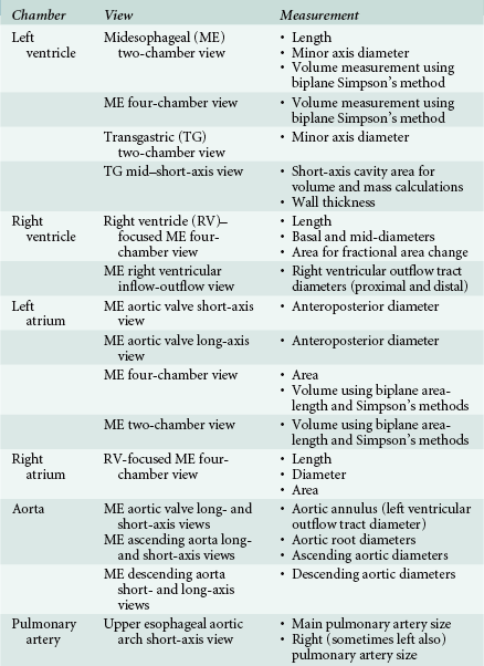
Table 11-1 summarizes the recommended views for performing various dimension and flow measurements during TEE.
 Measurement of Cardiac Chamber Dimensions
Left Ventricle
Left ventricular systolic function is a key determinant of clinical outcomes in almost every illness affecting the heart. Consequently, assessing left ventricular size and thereby its systolic function is one of the most important goals of any echocardiographic examination. No echocardiogram can be considered complete without an assessment of left ventricular size and systolic function. 12
Left Ventricular Linear Dimensions
Earlier guidelines recommended that the measurements be performed using the leading edge–to–leading edge technique. 13 This technique was required because the spatial resolution of the grayscale images at that time was insufficient for accurate delineation of the tissue/blood interfaces. Improvements in echocardiographic instrumentation have now made it possible to accurately identify actual tissue/blood interfaces, so most dimension measurements are currently performed using the inner edge–to–inner edge technique, which allows for measurements of the true cavity size. 12
During TEE, the left ventricular minor axis dimension can be obtained either from the midesophageal (ME) two-chamber view or from the transgastric (TG) two-chamber view ( Figs. 11-1 and 11-2, Videos 11-1 and 11-2  ). To obtain the ME two-chamber view, a proper ME four-chamber view (0 degrees) first needs to be obtained. From this position, advancement of the omniplane angle forward to 80 to 100 degrees while keeping the probe tip still and the mitral valve in the center will result in the ME two-chamber view. A slight retroflexion of the tip may be required to direct the imaging plane through the long axis of the left ventricle (LV) (see Video 11-1
  ) . The left ventricular diameter is then measured as the distance between the inferior and anterior walls at the level of the mitral leaflet tips.
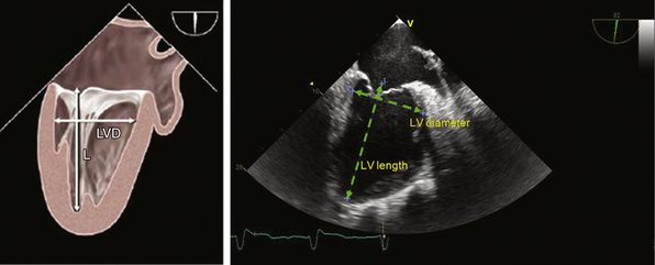
Figure 11-1 Measurement of left ventricular (LV) length and minor axis diameter from midesophageal two-chamber view. L, Length; LVD, left ventricular diameter. (Modified with permission from Lang RM, Bierig M, Devereux RB, et al. Recommendations for chamber quantification: a report from the American Society of Echocardiography’s Guidelines and Standards Committee and the Chamber Quantification Writing Group, developed in conjunction with the European Association of Echocardiography, a branch of the European Society of Cardiology. J Am Soc Echocardiogr. 2005;18:1440-1463.)
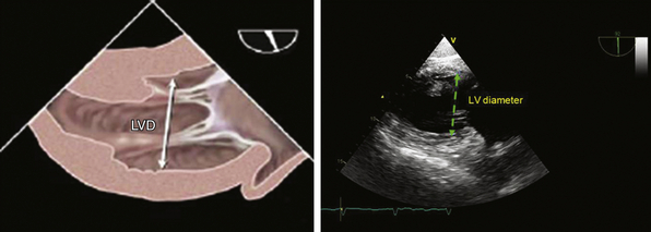
Figure 11-2 Measurement of left ventricular minor axis diameter from transgastric two-chamber view. LVD, Left ventricular diameter. (Modified with permission from Lang RM, Bierig M, Devereux RB, et al. Recommendations for chamber quantification: a report from the American Society of Echocardiography’s Guidelines and Standards Committee and the Chamber Quantification Writing Group, developed in conjunction with the European Association of Echocardiography, a branch of the European Society of Cardiology. J Am Soc Echocardiogr. 2005;18:1440-1463.)
The TG two-chamber view can be obtained from the TG mid–short-axis view (0 degrees) by advancing the omniplane angle forward to 80 to 90 degrees. A slight anteflexion of the transducer tip may be required to make the LV horizontal (see Video 11-2  ). The measurement is then performed in the same manner as described previously.
The left ventricular length or major axis dimension is the distance between the midpoint on the mitral annular plane and the left ventricular apex. During TTE, this dimension is usually obtained from the apical four-chamber view. However, its analogous view during TEE—the ME four-chamber view—often results in foreshortening of the LV, so the ME two-chamber view is preferred for measuring left ventricular length during TEE (see Fig. 11-1). 12 It is usually not possible to obtain the same measurement from the TG two-chamber view, because the left ventricular apex is almost invariably excluded from the image sector.
Reference ranges and partition values for left ventricular linear dimensions are presented in Table 11-2. For the reasons mentioned, these values have been derived only from transthoracic imaging; therefore, no such data exist for TEE. However, previous studies have shown that, when carefully performed, measurements obtained by TEE closely match those obtained from TTE.14,15 Thus, the American Society of Echocardiography recommends using the same reference ranges for left ventricular dimensions in TEE as well. 12
TABLE 11-2
Reference Ranges and Partition Values for Left Ventricle Size
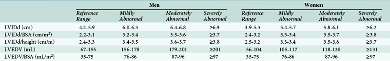
Data from Lang RM, Bierig M, Devereux RB, et al. Recommendations for chamber quantification: a report from the American Society of Echocardiography’s Guidelines and Standards Committee and the Chamber Quantification Writing Group, developed in conjunction with the European Association of Echocardiography, a branch of the European Society of Cardiology. J Am Soc Echocardiogr. 2005;18:1440-1463.
The major advantage of linear measurements is that they are simple, easy to perform, provide a quick estimate of the left ventricular size and, most importantly, have the least interobserver variability.16–18 However, because they are performed only in one dimension, linear measurements do not provide a true assessment of left ventricular size in the case of distorted ventricles, which are commonly observed in patients with coronary artery disease. Nevertheless, linear measurements have been shown to be reliable and have proven useful in clinical decision making regarding diseases affecting left ventricular symmetry, such as valvular heart disease, hypertension, and cardiomyopathies. 19
Left Ventricular Wall Thickness and Relative Wall Thickness
Left ventricular wall thickness is the end-diastolic thickness of the inferolateral wall and the interventricular septum. The recommended view for performing these measurements in TEE is the TG mid–short-axis view ( Fig. 11-3, Video 11-3  ). To obtain this view, the probe should be inserted into the stomach with the omniplane angle kept at 0 degrees. The probe should then be anteflexed and rotated to the right or left to develop the short-axis view of the LV and bring the LV to the center of the image. A slight advancement or withdrawal of the probe may be required to orient the imaging plane through the midportion of the ventricle, which can be recognized by the presence of papillary muscles. The grayscale image gain may have to be adjusted to optimize endocardial definition. From this view, the thicknesses of the inferolateral wall and septum are measured as shown in Figure 11-3.
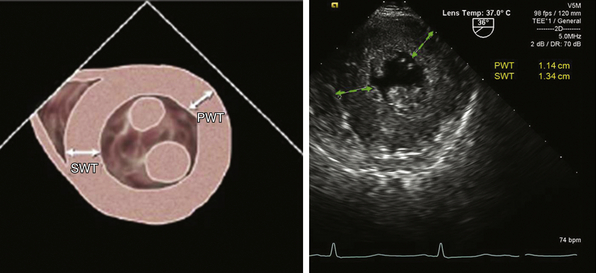
Figure 11-3 Measurement of left ventricular posterior wall and septal thickness from transgastric mid–short-axis view. PWT, Posterior wall thickness; SWT, septal wall thickness. (Modified with permission from Lang RM, Bierig M, Devereux RB, et al. Recommendations for chamber quantification: a report from the American Society of Echocardiography’s Guidelines and Standards Committee and the Chamber Quantification Writing Group, developed in conjunction with the European Association of Echocardiography, a branch of the European Society of Cardiology. J Am Soc Echocardiogr. 2005;18:1440-1463.)

where ILWIDd is the end-diastolic thickness of the inferolateral wall of the LV, and LVIDd is the diameter of the left ventricular cavity at end-diastole.
In patients with left ventricular hypertrophy (defined based on increased left ventricular mass as described later), an increased relative wall thickness (≥0.42) signifies concentric hypertrophy, whereas a normal relative wall thickness (<0.42) indicates the presence of eccentric hypertrophy.20,21 Concentric left ventricular hypertrophy is observed in conditions causing a pressure overload of the LV, such as hypertension, aortic stenosis, and coarctation of the aorta. In contrast, eccentric hypertrophy is common in diseases causing volume overload, such as aortic and mitral regurgitation. Eccentric hypertrophy is also observed during the late degenerative stages of diseases otherwise characterized by concentric hypertrophy, such as hypertrophic cardiomyopathy and aortic stenosis. Sometimes relative wall thickness is increased without a concomitant increase in left ventricular mass. This is known as concentric remodeling and generally occurs in response to pressure overload. The presence of concentric remodeling has been shown to be an adverse prognostic marker in certain disease conditions.22,23
The normal ranges and partition values for left ventricular wall thickness are presented in Table 11-3.
TABLE 11-3
Reference Ranges and Partition Values for Left Ventricular Wall Thickness and Mass
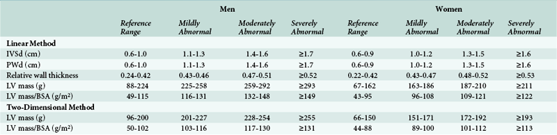
Data from Lang RM, Bierig M, Devereux RB, et al. Recommendations for chamber quantification: a report from the American Society of Echocardiography’s Guidelines and Standards Committee and the Chamber Quantification Writing Group, developed in conjunction with the European Association of Echocardiography, a branch of the European Society of Cardiology. J Am Soc Echocardiogr. 2005;18:1440-1463.
Left Ventricular Volume
Linear Method or Cubed Method

where LVID is the left ventricular internal dimension.

where LVEDV is the left ventricular end-diastolic volume, and LVESV is the left ventricular end-systolic volume.
Given that the cubed method assumes the LV to be spherical, which clearly is not true, it inevitably introduces errors into the estimation of left ventricular volume. Several modifications of this method have been proposed to correct for this error, such as the Teichholz and Quinones methods.24,25 The Teichholz method is given as 25

(Please note that for this equation, the LVID must be measured in centimeters.)
Two-Dimensional Methods
As mentioned, the cubed method, which is based on a single linear measurement of the LV, has significant limitations and cannot be applied in patients with regional WMAs. By incorporating left ventricular dimensions from more than one plane, 2D methods allow for more accurate estimation of left ventricular volume. There are two different 2D methods that can be used for this purpose: the area-length method and the biplane Simpson’s method. 12
The area-length method assumes the LV to be bullet-shaped ( Fig. 11-4). The volume is calculated using the following equation:

where area is the cross-sectional area of the left ventricular cavity measured at the mid-ventricle level, and length is the left ventricular long-axis length as described previously.
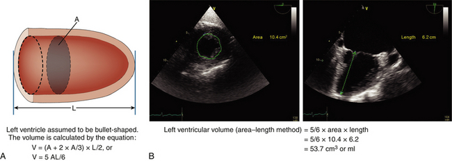
Figure 11-4 A and B, Measurement of left ventricular volume using area-length method. Left ventricular cavity cross-sectional area (A) is measured from transgastric mid–short-axis view, and length (L) is measured from midesophageal two-chamber view. Note that papillary muscles are considered to be part of left ventricular cavity. Volume in example will be 53.7 mL (⅚ × 10.4 × 6.2).
The biplane Simpson’s method overcomes many of the geometric assumptions associated with the aforementioned methods. This method divides the entire left ventricular cavity into a stack of elliptical discs (usually 20), and the volume of the left ventricular cavity is calculated by summation of the volumes of each of these discs ( Fig. 11-5). The volume of each disc is calculated as the cross-sectional area of the disc multiplied by its height. The cross-sectional area is computed from the two orthogonal diameters obtained from the four-chamber and two-chamber views, and the height is derived from the length of the LV. All of these calculations are performed automatically using built-in software available in all modern echocardiographic equipment.
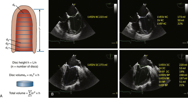
Figure 11-5 A and B, Measurement of left ventricular volume using biplane Simpson’s method. Endocardial border is traced in midesophageal four-chamber and two-chamber views at end-diastole and end-systole. 2C, Two-chamber; 4C, four-chamber; BP, biplane; EDV, end-diastolic volume; EF, ejection fraction; ESV, end-systolic volume; LV, left ventricular; SV, stroke volume. (Modified with permission from Feigenbaum H, Armstrong W, Ryan T, eds. Feigenbaum’s Echocardiography. 6th ed. Philadelphia: Lippincott Williams & Wilkins; 2005.)
While performing these measurements, great caution must be exercised to ensure that the left ventricular cavity is not foreshortened. Slight retroflexion of the tip of the transducer to bring the true left ventricular apex into view may help avoid foreshortening (Video 11-4  ), but it may still be difficult to obtain a non-foreshortened view of the LV in the ME four-chamber view.
The biplane Simpson’s method is currently the most accurate (and the recommended) 2D echocardiographic method for estimating left ventricular volume because it employs the fewest mathematical assumptions regarding the left ventricular cavity shape and also corrects for distortion of left ventricular geometry. 12 However, the accuracy of this method is highly dependent on adequate endocardial border delineation. As already described, the echocardiography machine settings should be adjusted to obtain the best possible endocardial delineation. If, despite these adjustments, the endocardial border cannot be visualized adequately in one of the two requisite views, the single-plane Simpson’s method can be used to obtain left ventricular volumes. However, this method will not be accurate enough in the presence of significant regional WMAs. When the endocardial border cannot be adequately visualized in either of the two views, the Simpson’s method should be abandoned and the area-length method used to estimate left ventricular volume.
Table 11-2 describes the normal ranges and partition values of left ventricular volumes derived from 2D methods.
Three-Dimensional Methods
The recent advent of three-dimensional (3D) echocardiography has significantly improved our ability to accurately estimate left ventricular volumes by eliminating the need for mathematical assumptions regarding the shape of the LV. The left ventricular cavity can be directly imaged in a 3D space, and its volume can be accurately calculated. Comparative studies using magnetic resonance imaging (MRI) as the gold standard have shown excellent agreement between the two techniques and have demonstrated 3D echocardiography to be superior to 2D echocardiography for estimating left ventricular volumes.26–30 The availability of live 3D TEE has further improved image quality, and the application of quantitative techniques to these images has the potential to provide an even more accurate estimation of left ventricular volumes than ever before. However, a detailed description of these techniques, including their advantages and potential pitfalls, is beyond the scope of this chapter.
Left Ventricular Mass
Left ventricular hypertrophy is an important prognosis determinant in a number of clinical conditions such as hypertension, aortic stenosis, aortic regurgitation, and cardiomyopathies.21,31–36 Accordingly, the presence and extent of left ventricular hypertrophy forms the basis of many of the key therapeutic decisions in these disease states. Echocardiography, by allowing for estimation of left ventricular mass, is the most clinically relevant tool for detection and characterization of left ventricular hypertrophy.36–38 Assessing left ventricular mass via echocardiography has been extensively used in clinical and research settings for prognostication, guiding treatment, and following the effects of various pharmacologic and nonpharmacologic measures aimed at bringing about regression of left ventricular hypertrophy.31,36–39
Linear Method
where 1.04 is the myocardial density, and 0.8 is the correction factor. LVIDd, IVSd, and ILWd represent the end-diastolic left ventricular internal diameter, interventricular septal thickness, and inferolateral wall thickness, respectively.
Two-Dimensional Methods
For the area-length method ( Fig. 11-6), the TG mid–short-axis view is obtained at the papillary muscle level, and the left ventricular epicardial and endocardial cross-sectional areas (A1 and A2) are measured by tracing the epicardium and endocardium, respectively. When tracing the endocardium, the papillary muscles are included in the cavity, not in the myocardium. Left ventricular length (L) is then measured in the ME two-chamber view as previously described. Left ventricular mass is then calculated using the following equation:
where t is the mean wall thickness derived by subtracting the left ventricular cavity radius from the left ventricular radius as described in the equation:
In the example shown in Figure 11-6, B, t would be 1.16 cm [√(27.8/3.14) − √(10.4/3.14)]. Inserting all the values into the equation will yield a left ventricular mass of 122.6 g.
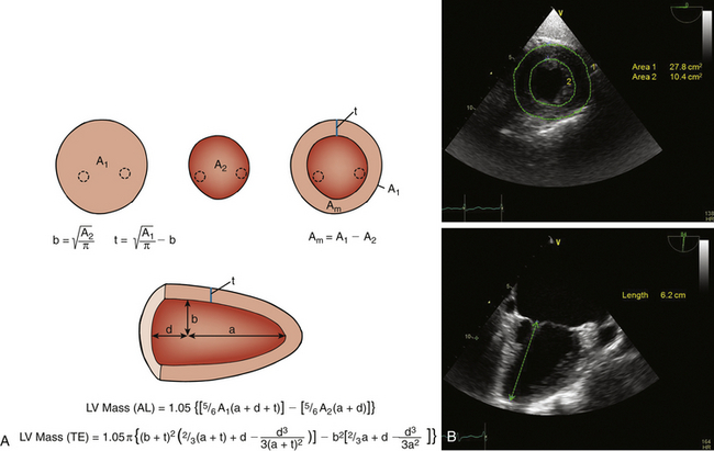
Figure 11-6 A and B, Estimation of left ventricular (LV) mass using area-length (AL) formula and truncated-ellipsoid (TE) formula. See text for details. A1, Total LV area; A2, LV cavity area; Am, myocardial area; a, length of LV from widest minor axis radius to apex; b, short-axis radius of LV cavity (back-calculated from short-axis cavity area); d, length of LV from widest minor axis radius to mitral annulus plane; t, mean wall thickness. (Modified with permission from Schiller NB, Shah PM, Crawford M, et al. Recommendations for quantitation of the left ventricle by two-dimensional echocardiography. American Society of Echocardiography Committee on Standards, Subcommittee on Quantitation of Two-Dimensional Echocardiograms. J Am Soc Echocardiogr. 1989;2:358-367.)
An alternate method for estimating left ventricular mass is based on the truncated ellipsoid method (see Fig. 11-6, A) and can be calculated with the following equation:
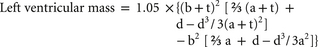
where b is the left ventricular cavity radius, which is back-calculated from the area as √(A2/π), and a and d
Stay updated, free articles. Join our Telegram channel

Full access? Get Clinical Tree


