Sound is a mechanical vibration transmitted through an elastic medium. When it propagates through air at the appropriate frequency, sound may produce the sensation of hearing. Ultrasound includes that portion of the sound spectrum having a frequency greater than 20,000 cycles per second (20 KHz), which is considerably above the audible range of human hearing. The use of ultrasound to study the structure and function of the heart and great vessels defines the field of echocardiography. The production of ultrasound for diagnostic purposes involves complex physical principles and sophisticated instrumentation. As technology has evolved, a thorough understanding of these principles mandates an extensive background in physics and engineering. Fortunately, the use of echocardiography for clinical purposes does not require a complete mastery of the physics and instrumentation involved in the creation of the ultrasound image. However, a basic understanding of these facts is necessary to take full advantage of the technique and to appreciate the strengths and limitations of the technology.
This book is intended principally as a clinical guide to the broad field of echocardiography, to be used by clinicians, students, and sonographers concerned more about the practical application of the technology than the underlying physics. For this reason, an extensive description of the physics and engineering of ultrasound is beyond the scope of this book. Instead, this chapter focuses on those aspects of physics and instrumentation that are relevant to the understanding of ultrasound and its practical application to patient care. In addition, many of the newer technical advances in ultrasound instrumentation are presented briefly, primarily to provide the reader a sense of the changing and ever-improving nature of echocardiography.
Physical Principles
Ultrasound (in contrast to lower, i.e., audible frequency sound) has several characteristics that contribute to its diagnostic utility. First, ultrasound can be directed as a beam and focused. Second, as ultrasound passes through a medium, it obeys the laws of reflection and refraction. Finally, targets of relatively small size reflect ultrasound and can, therefore, be detected and characterized. A major disadvantage of ultrasound is that it is poorly transmitted through a gaseous medium and attenuation occurs rapidly, especially at higher frequencies. As a wave of ultrasound propagates through a medium, the particles of the medium vibrate parallel to the line of propagation, producing longitudinal waves. Thus, a sound wave is characterized by areas of more densely packed particles within the medium (an area of compression) alternating with regions of less densely packed particles (an area of rarefaction). The amount of reflection, refraction, and attenuation depends on the acoustic properties of the various media through which an ultrasound beam passes. Tissues composed of solid material interfaced with gas (such as the lung) will reflect most of the ultrasound energy, resulting in poor penetration. Very dense media also reflect a high percentage of the ultrasound energy. Soft tissues and blood allow relatively more ultrasound energy to be propagated, thereby increasing penetration and improving diagnostic utility. Bone also reflects most ultrasound energy, not because it is dense but because it contains so many interfaces.
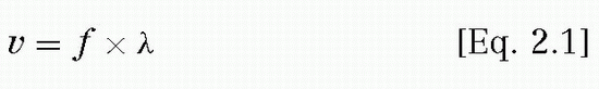
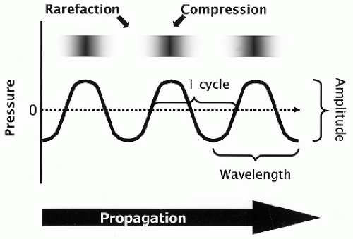
The ultrasound wave is often graphically depicted as a sine wave in which the peaks and troughs represent the areas of compression and rarefaction, respectively (Fig. 2.1). Small pressure changes occur within the medium, corresponding to these areas, and result in tiny oscillations of particles, although no actual particle motion occurs. Depicting ultrasound in the form of a sine wave has some limitations but allows the demonstration of several fundamental principles. The sum of one compression and one rarefaction represents one cycle, and the distance between two similar points along the wave corresponds to wavelength (see Table 2.1 for definitions of commonly used terms). Over the range of diagnostic ultrasound, wavelength varies from approximately 0.15 to 1.5 mm in soft tissue. The frequency of the sound wave is the number of wavelengths per unit of time. Thus, wavelength and frequency are inversely related and their product represents the velocity of the sound wave:
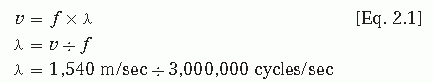
where v is velocity, f is frequency (in cycles per second or hertz), and λ is wavelength. Velocity through a given medium depends on the density and elastic properties or stiffness of that medium. Velocity is directly related to stiffness and inversely related to density. Ultrasound travels faster through a stiff medium, such as bone. Velocity also varies with temperature, but because body temperature is maintained within a relatively narrow range, this is of little significance in medical imaging. Table 2.2 provides a comparison of average velocity values in various types of tissues. Within soft tissue, velocity of sound is fairly constant at approximately 1,540 m/sec (or 1.54 m/msec, or 1.54 mm/µsec). Thus, to find the wavelength of a 3.0-MHz transducer, the solution would be given by
FIGURE 2.1. This schematic illustrates how sound can be depicted as a sine wave in which peaks and troughs correspond to areas of compression and rarefaction, respectively. As sound energy propagates through tissue, the wave has a fixed wavelength that is determined by the frequency and amplitude that is a measure of the magnitude of pressure changes. See text for further details.
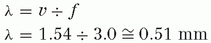
A simpler version of this equation is given by λ (in millimeters) = 1.54/f, where f is the transducer frequency (in megahertz). This converts 1,540 m/sec to 1.54 mm/µsec, expresses frequency in megahertz, and yields wavelength in millimeters. Thus,
Table 2.1 Definitions of Basic Terms
Term
Definition
Absorption
The transfer of ultrasound energy to the tissue during propagation
Acoustic impedance
The product of the density of the medium and the velocity of sound; differences in acoustic impedance between two media determine the ratio of transmitted versus reflected sound at the interface
Amplitude
The magnitude of the pressure changes along the wave; also, the strength of the wave (in decibels)
Attenuation
The net loss of ultrasound energy as a wave propagates through a medium
Cycle
The combination or sum of one compression and one rarefaction of a propagating wave
Dead time
The time in between pulses that the echograph is not emitting ultrasound
Decibel
A logarithmic measure of the intensity of sound, expressed as a ratio to a reference value (dB)
Duty factor
The fraction of time that the transducer is emitting ultrasound, a unitless number between 0 and 1
Far field
The diverging conical portion of the beam beyond the near field
Frequency
The number of cycles per second, measured in Hertz (Hz)
Gain
The degree, or percentage, of amplification of the returning ultrasound signal
Half-layer value
The distance an ultrasound beam penetrates into a medium before its intensity has attenuated to one half the original value
Intensity
The concentration or distribution of power within an area, often the cross-sectional area of the ultrasound beam, analogous to loudness
Longitudinal wave
A cyclic disturbance in which the energy propagation is parallel to the direction of particle motion
Near field
The proximal cylindrical-shaped portion of the ultrasound beam before divergence begins to occur
Period
The time required to complete one cycle, usually expressed in microseconds (µsec)
Piezoelectricity
The phenomenon of changing shape in response to an applied electric current, resulting in vibration and the production of sound waves; the ability to produce an electric impulse in response to a mechanical deformation; thus, the interconversion of electrical and sound energy
Power
The rate of transfer over time of the acoustic energy from the propagating wave to the medium, measured in Watts
Pulse
A burst or packet of emitted ultrasound of finite duration, containing a fixed number of cycles traveling together
Pulse length
The physical length or distance that a pulse occupies in space, usually expressed in millimeters (mm)
Pulse repetition frequency
The rate at which pulses are emitted from the transducer, i.e., the number of pulses emitted within a period of time, usually 1 second
Resolution
The smallest distance between two points that allows the points to be distinguished as separate
Sensitivity
The ability of the system to image small targets at a given depth
Ultrasound
A mechanical vibration in a physical medium, characterized by a frequency >20,000 Hz
Velocity
The speed at which sound moves through a given medium
Wavelength
The length of a single cycle of the ultrasound wave; a measure of distance, not time
If an ultrasound wave encounters an area of higher elasticity or stiffness, for example, velocity will increase. Because frequency does not change, wavelength will also increase. As is discussed later, wavelength is a determinant of resolution: the shorter the wavelength, the smaller the target that is able to reflect the ultrasound wave and thus the greater the resolution.
Table 2.2 Velocity of Sound in Air and Various Types of Tissues
Medium
Velocity (m/sec)
Air
330
Fat
1,450
Water
1,480
Soft tissue
1,540
Kidney
1,560
Blood
1,570
Muscle
1,580
Bone
4,080
Another fundamental property of sound is amplitude, which is a measure of the strength of the sound wave (Fig. 2.1). It is defined as the difference between the peak pressure within the medium and the average value, depicted as the height of the sine wave above and below the baseline. Amplitude is measured in decibels, a logarithmic unit that relates acoustic pressure to some reference value. The primary advantage of using a logarithmic scale to display amplitude is that a very wide range of values can be accommodated and weak signals can be displayed along side much stronger signals. Of practical use, an increase of 6 dB is equal to a doubling of signal amplitude, and 60 dB represents a 1,000-fold change in amplitude or loudness. A parameter closely related to amplitude is power, which is defined as the rate of energy transfer to the medium, measured in watts. For clinical purposes, power is usually represented over a given area (often the beam area) and referred to as intensity (watts per centimeter squared or W/cm2). This is analogous to loudness. Intensity diminishes rapidly with propagation distance and has important implications with respect to the biologic effects of ultrasound, which are discussed later.
Interaction Between Ultrasound and Tissue
These basic characteristics of ultrasound have practical implications for the interaction between ultrasound and tissue. For example, the higher the frequency of the ultrasound wave (and the shorter the wavelength), the smaller the structures that can be accurately resolved. Because precise identification of small structures is a goal of imaging, the use of high frequencies would seem desirable. However, higher frequency ultrasound has less penetration compared with lower frequency ultrasound. The loss of ultrasound as it propagates through a medium is referred to as attenuation. This is a measure of the rate at which the intensity of the ultrasound beam diminishes as it penetrates the tissue. Attenuation has three components: absorption, scattering, and reflection. Attenuation always increases with depth and is also affected by the frequency of the transmitted beam and the type of tissue through which the ultrasound passes. The higher the frequency, the more rapidly it will attenuate. Attenuation may be expressed as the “half-value layer” or the “half-power distance,” which is a measure of the distance that ultrasound travels before its amplitude is attenuated to one half its original value. Representative half-power distances are listed in Table 2.3. As a rule of thumb, the attenuation of ultrasound in tissue is between 0.5 and 1.0 dB/cm/MHz. This approximation describes the expected loss of energy (in decibels) that would occur over the round-trip distance that a beam would travel after being emitted by a given transducer. For example, if a 3-MHz transducer is used to image an object at a depth of 12 cm (24-cm round trip), the returning signal could be attenuated as much as 72 dB (or nearly 4,000-fold). As expected, attenuation is greater in soft tissue compared with blood and is even greater in muscle, lung, and bone.
Table 2.3 Representative Half-Power Distances Relevant to Echocardiography
Material
Half-Power Distance (cm)
Water
380
Less attenuation
Blood
15
Soft tissue (except muscle)
1-5
Muscle
0.6-1
Bone
0.2-0.7
Air
0.08
Lung
0.05
More attenuation
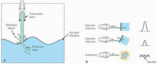
The velocity and direction of the ultrasound beam as it passes through a medium are a function of the acoustic impedance of that medium. Acoustic impedance (Z, measured in rayls) is simply the product of velocity (in meters per second) and physical density (in kilograms per cubic meter). Within a homogeneous structure, the density and stiffness of the medium primarily determine the behavior of a transmitted ultrasound beam. In such a structure, sound would travel in a straight line at a constant velocity, depending on the density and stiffness. Variations in impedance create an acoustic mismatch between regions. The greater the acoustic mismatch, the more the energy reflected rather than transmitted. Within the body, the tissues through which an ultrasound beam passes have different acoustic impedances. When the beam crosses a boundary between two tissues, a portion of the energy is reflected, a portion is refracted, and a portion continues in a relatively straight line (Fig. 2.2A).
FIGURE 2.2. A: A transmitted wave interacts with an acoustic interface in a predictable way. Some of the ultrasound energy is reflected at the interface and some is transmitted through the interface. The transmitted portion of the energy is refracted, or bent, depending on the angle of incidence and differences in impedance between the tissues. B: The interaction between an ultrasound wave and its target depends on several factors. A specular reflection occurs when ultrasound encounters a target that is large relative to the transmitted wavelength. The amount of ultrasound energy that is reflected to the transducer by a specular target depends on the angle and the impedance of the tissue. Targets that are small relative to the transmitted wavelength produce a scattering of ultrasound energy, resulting in a small portion of energy being returned to the transducer. This type of interaction results in “speckle” that produces the texture within tissues.
These interactions between the ultrasound beam and the acoustic interfaces form the basis for ultrasound imaging. The phenomena of reflection and refraction obey the laws of optics and depend on the angle of incidence between the transmitted beam and the acoustic interface as well as on the acoustic mismatch, that is, the magnitude of the difference in acoustic impedance. Small differences in velocity also determine refraction. These properties explain the importance of using an acoustic coupling gel during transthoracic imaging. Without the gel, the air-tissue interface at the skin surface results in more than 99% of the ultrasonic energy being reflected at this level. This is primarily due to the very low acoustic impedance of air. The use of gel between the transducer and the skin surface greatly increases the percentage of energy that is transmitted into and out of the body, thereby allowing imaging to occur.
As the ultrasound beam is transmitted through tissue, it encounters a complex array of large and small interfaces and targets, each of which affect the transmission of the ultrasound energy. These interactions can be broadly categorized as specular echoes and scattered echoes (Fig. 2.2B). Specular echoes are produced by reflectors that are large relative to ultrasound wavelength, such as the endocardial surface of the left ventricle. Such targets reflect a relatively greater proportion of the ultrasound energy in an angle-dependent fashion. The spatial orientation and the shape of the reflector determine the angles of specular echoes. Examples of specular reflectors include endocardial and epicardial surfaces, valves, and pericardium.
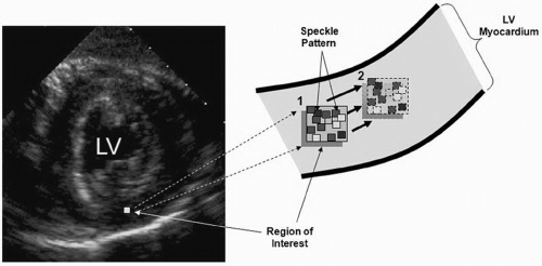
FIGURE 2.3. This schematic demonstrates how speckle tracking is performed. In this simplified example, a single region of interest in the posterior left ventricular (LV) wall is tracked based on its unique speckle signature. In the drawing, a small region in the midmyocardium moves over time from point 1 to point 2.
Targets that are small relative to the wavelength of the transmitted ultrasound produce scattering, and such objects are sometimes referred to as Rayleigh scatterers. The resultant echoes are diffracted or bent and scattered in all directions. Because the percentage of energy returning to the transducer from scattered echoes is considerably less than that resulting from specular interactions, the amplitude of the signals produced by scattered echoes is very low (Fig. 2.2B). Despite this fact, scattering has important clinical significance (for both echocardiography and Doppler imaging). Scattered echoes contribute to the visualization of surfaces that are parallel to the ultrasonic beam and also provide the substrate for visualizing the texture of gray-scale images. The term speckle is used to describe the tissue-ultrasound interactions that result from a large number of small reflectors within a resolution cell. Without the ability to record scattered echoes, the left ventricular wall, for example, would appear as two bright linear structures, the endocardial and the epicardial surfaces, with nothing in between.
Because the distribution of speckle within a small region of interest is random but fairly constant, if such regions could be identified, they could be tracked over time and space. By exploiting this phenomenon, a region within the myocardium can be followed throughout the cardiac cycle, a technique referred to as speckle tracking. This method, for example, allows rotational motion (or torsion) of the left ventricular myocardium to be detected and quantified (Fig. 2.3). And, because this is not a Doppler technique, it is not angle-dependent.
From the above discussion, it is evident that the interaction between an ultrasound beam and a reflector depends on the relative size of the targets and the wavelength of the beam. If a solid object is submerged in water, for example, whether reflection of ultrasound occurs depends on the size of the object with respect to the wavelength of the transmitted ultrasound. Specifically, the thickness or profile of the object relative to the ultrasound beam must be at least one-fourth the wavelength of the ultrasound. Thus, as the size of the target decreases, the wavelength of the ultrasound must decrease proportionately to produce a reflection and permit the object to be recorded. This explains why higher frequency ultrasound allows smaller objects to be visualized. In clinical practice, echocardiography typically employs ultrasound with a range of 2,000,000 to 8,000,000 cycles per second (2-8 MHz). At a frequency of 2 MHz, it is generally possible to record distinct echoes from interfaces separated by approximately 1 mm. However, because high-frequency ultrasound is reflected by many small interfaces within tissue, resulting in scattering, much of the ultrasonic energy becomes attenuated and less energy is available to penetrate deeper into the body. Thus, penetration is reduced as frequency increases. Similarly, as the medium becomes less homogeneous, the degree of reflection and refraction increases, resulting in less penetration of the ultrasound energy.
The Transducer
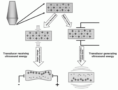
The use of ultrasound for imaging became practical with the development of piezoelectric transducers. The principles of piezoelectricity are illustrated in Figure 2.4. Piezoelectric substances or crystals rapidly change shape or vibrate when an alternating electric current is applied. It is the rapidly alternating expansion and contraction of the crystal material that produces the sound waves. Equally important is the fact that a piezoelectric crystal will produce an electric impulse when it is deformed by reflected sound energy. Such piezoelectric crystals form the critical component of ultrasound transducers. Although a variety of piezoelectric materials exist, most commercial transducers employ ceramics, such as ferroelectrics, barium titanate, and lead zirconate titanate. The creation of an ultrasound pulse thus requires that an alternating electric current be applied to a piezoelectric element. This results in the emission of sound energy from the transducer, followed by a period of quiescence during which the transducer “listens” for some of the transmitted ultrasound energy to be reflected back (known as “dead time”). The amount of acoustic energy that returns to the transducer is a measure of the strength and depth of the reflector. The time required for the ultrasound pulse to make the round-trip from transducer to target and back again allows calculation of the distance between the transducer and the reflector.
An ultrasound transducer consists of many small, carefully arranged piezoelectric elements that are interconnected electronically. The frequency of the transducer is determined by the thickness of these elements. Each element is coupled to electrodes, which transmit current to the crystals, and then record the voltage generated by the returning signals. An important component of transducer design is the dampening (or backing) material, which shortens the ringing response of the piezoelectric material after the brief excitation pulse. An excessive ringing response (or “ringdown”) lengthens the ultrasonic pulse and decreases range resolution. Thus, the dampening material both shortens the ringdown and provides absorption of backward and laterally transmitted acoustic energy. At the surface of the transducer, matching layers are applied to provide acoustic impedance matching between the piezoelectric elements and the body. This increases the efficiency of transmitted energy by minimizing the reflection of the ultrasonic wave as it exits the transducer surface.
FIGURE 2.4. The principles of piezoelectricity. A piezoelectric crystal will vibrate when an electric current is applied, resulting in the generation and transmission of ultrasound energy. Conversely, when reflected energy encounters a piezoelectric crystal, the crystal will change shape in response to this interaction and produce an electrical impulse. See text for further details.
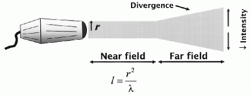
Transducer design is critically important to optimal image creation. An important feature of ultrasound is the ability to direct or focus the beam as it leaves the transducer. This results in a parallel and cylindrically shaped beam. Eventually, however, the beam diverges and becomes cone shaped (Fig. 2.5). The proximal or cylindrical portion of the beam is referred to as the near field or Fresnel zone. When it begins to diverge, it is called the far field or Fraunhofer zone. For a variety of reasons, imaging is optimal within the near field. Thus, maximizing the length of the near field is an important goal of echocardiography.
FIGURE 2.5. When ultrasound is emitted from a transducer, the shape of the beam behaves in a predictable manner. If the transducer face is round, the transmitted beam will remain cylindrical for a distance, defined as the near field. After propagating for a certain distance, the beam will begin to diverge and become cone shaped. This region of the beam is referred to as the far field. Within this portion of the beam, a decrease in intensity occurs. The length of the near field is determined by the radius of the transducer face and the wavelength or frequency of the transmitted energy. See text for details.
The length of the near field (l) is described by the formula:
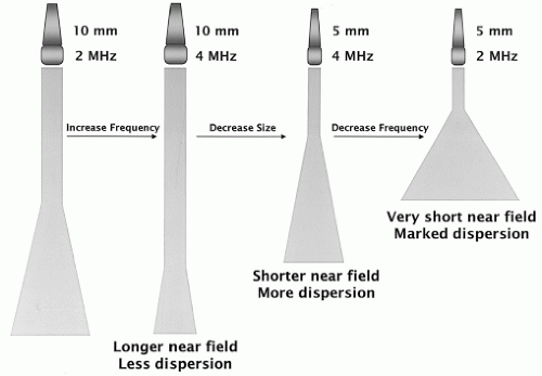
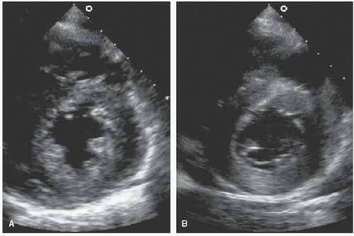
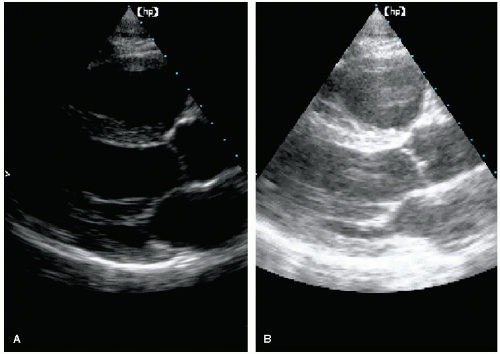
where r is the radius of the transducer and λ is the wavelength of the emitted ultrasound. Either decreasing the wavelength (increasing the frequency) or increasing the size of the transducer will lengthen the near field. These relationships are illustrated in Figure 2.6. From the above formula, one might conclude that optimal ultrasound imaging would always employ a large-diameter, high-frequency transducer to maximize the length of the near field. Several factors prevent this approach from being practical. First, the transducer size is predominantly limited by the size of the intercostal spaces. A transducer that is too large will not be able to image between the ribs. Second, although higher frequency does lengthen the near field, it also results in greater attenuation and lower penetration of the ultrasound energy, thereby limiting its usefulness. These tradeoffs must be balanced to maximize imaging performance. Even when the near field length is maximized, most targets will still lie in the far field. To improve imaging in this area, the rate of beam divergence must be minimized. To decrease the amount of divergence in the far field, a large-diameter, high-frequency transducer is optimal. As discussed previously, focusing of the transmitted beam tends to improve imaging in the near field but will increase the rate or angle of divergence in the far field (Fig. 2.7). Focusing is accomplished through the use of an acoustic lens placed on the surface of the transducer or by constructing the piezoelectric crystal in a concave shape. Thus, transducer frequency, size, and focusing all interact to affect image quality in the near and far fields. Tradeoffs exist that must be taken into account to create optimal images. Figure 2.8 is an example of the effects of varying transducer frequencies on image quality and appearance. On the left, a short-axis view is recorded using a 3.0-MHz transducer. On the right, a similar image is captured using a 5.0-MHz probe. Note how the higher frequency results in improved resolution and detail, especially within the myocardium.
FIGURE 2.6. The length of the near field depends on transducer frequency and transducer size, as illustrated in these four examples. On the left, a transducer with a 10-mm diameter emits ultrasound at 2.0 MHz. This determines both the length of the near field and the rate of divergence in the far field. If the same size transducer emits energy at 4 MHz, the length of the near field increases and the rate of dispersion is less. A transducer half that size (5 mm) transmitting at 4.0 MHz will have a shorter near field. Finally, a 5-mm transducer that transmits at 2 MHz will have the shortest near field and the greatest rate of dispersion in the far field.
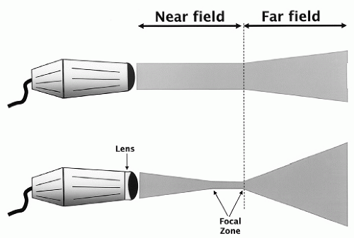
FIGURE 2.7. The ultrasound beam emitted by a transducer can be either unfocused (top) or focused by use of an acoustic lens (bottom). Focusing results in a narrower beam but does not change the length of the near field. An undesirable effect of focusing is that the rate of dispersion in the far field is greater.
FIGURE 2.8. The effects of different transducer frequencies on image quality and appearance. A: A 3.0-MHz transducer is used to record a short-axis view. B: The same image is recorded using a 5.0-MHz transducer.
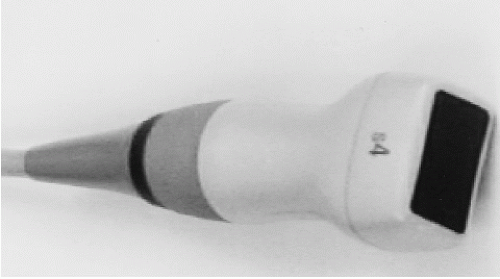
FIGURE 2.9. A phased-array ultrasound transducer.
Manipulating the Ultrasound Beam
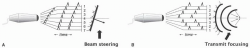
For most clinical applications, the ultrasound beam is both focused and steered electronically. Although beam manipulation can be done mechanically, with modern equipment, it is almost always achieved through the use of phased-array transducers, which consist of a series of small piezoelectric elements interconnected electronically (Fig. 2.9). In such transducers, the wave front of the beam consists of the sum of the individual wavelets produced by each element. By manipulating the timing of excitation of individual elements, both focusing and steering are possible. If all elements are excited simultaneously, each one will produce a circular wavelet that combines to generate a longitudinal wave front that is parallel to the face of the transducer and propagates in a direction perpendicular to that face. By adjusting the timing of excitation, as shown in Figure 2.10A, the beam can be steered. Further adjustments in the timing allow the beam to be steered through a sector arc, resulting in a two-dimensional image. Using a similar approach, electronic transmit focusing of the beam is also possible (Fig. 2.10B). For example, by exciting the outside elements first and then progressively activating the more central elements, the individual wavelets form a curved front that allows focusing at a particular distance within the near field. This can either be fixed or adjustable, and the process is referred to as dynamic transmit focusing.
FIGURE 2.10. A: Phased-array technology permits steering of the ultrasound beam. By adjusting the timing of excitation of the individual piezoelectric crystals, the wave front of ultrasound energy can be directed, as shown. Beam steering is a fundamental feature of how two-dimensional images are created. B: By adjusting the timing of excitation of the individual crystals within a phased-array transducer, the beam can be focused. In this example, the outer elements are fired first, followed sequentially by the more central elements. Because the speed of sound is fixed, this manipulation in the timing of excitation results in a wave front that is curved and focused. This is called transmit focusing.
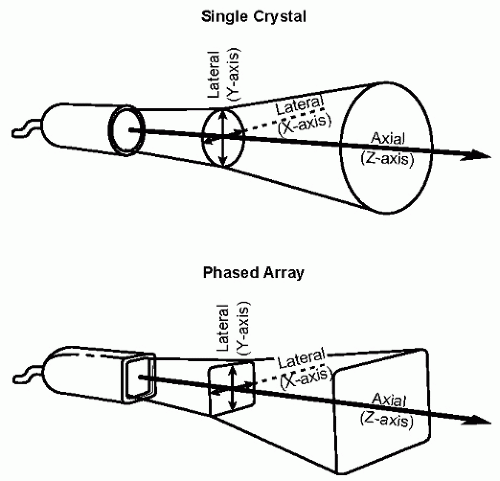
It should be recognized that the ultrasound beam is a three-dimensional structure that, in the case of a phased-array transducer, is roughly rectangular in cross section (Fig. 2.11). The dimensions of the beam are referred to as axial (along the axis of wave propagation) and lateral (parallel to the face of the transducer, sometimes called azimuthal). The lateral dimension is further divided into a vertical component and a horizontal component. Acoustic focusing through a lens will change the shape in the vertical and horizontal dimensions equally. Electronic focusing will narrow the beam in one of these two dimensions, resulting in a “thinner” sector slice. Transducers that employ annular phased-array technology have the capacity to focus in both dimensions, resulting in a compact, high-intensity beam profile.
FIGURE 2.11. The ultrasound beam can be represented as a three-dimensional structure. A single-crystal transducer (top) will emit a cylindrically shaped beam. If the transducer face is rectangular shaped (bottom), the beam will also have a rectangular shape. The various beam axes are labeled in the two drawings.
Another type of transducer uses a linear array of elements. Such transducers have a rectangular face with crystals aligned parallel to one another along the length of the transducer face. Unlike phased-array transducers, the elements are excited simultaneously, so the individual scan lines are directed perpendicular to the face and remain parallel to each other. This results in a rectangle-shaped beam that is unfocused. Linear-array technology is often used for abdominal, vascular, or obstetric applications. Alternatively, the face of a linear transducer can be curved to create a sector scan. This innovative design is now being used in some handheld ultrasound devices.
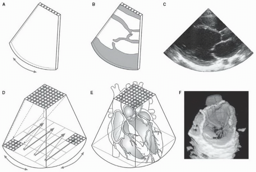
To perform real-time three-dimensional echocardiography, a more complex transducer design is needed. This requires the arrangement of the piezoelectric elements into a two-dimensional matrix. Each element represents a scan line that is used to construct the three-dimensional data set. For example, if the matrix consists of 64 by 64 elements, 4,096 scan lines can be generated. Through careful manipulation of the timing of excitation, a pyramidal-shaped volume (rather than a tomographic slice) of ultrasound data can be collected. By interrogating the volumetric shape several times (>20) per second, real-time imaging in three dimensions is possible (Fig. 2.12). This is covered in greater detail in Chapter 3.
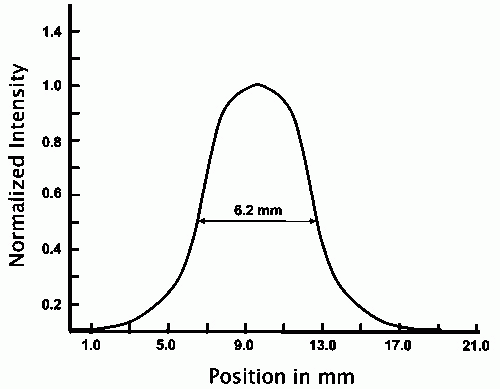
Focusing has the effect of concentrating the acoustic energy into a smaller area, resulting in increased intensity at the point of focus. Intensity also varies across the lateral dimensions of the beam, being greatest at the center and decreasing in intensity toward the edges. When the shape of the ultrasonic beam is diagrammed, it is conventional to draw the edge of the beam to the half-value limit of the beam plot. An example of a transaxial beam plot is illustrated in Figure 2.13. This diagram illustrates the important relationship between intensity and beam width. At its peak intensity, the beam may be as narrow as 1 mm. At its weakest intensity, however, beam width may be as great as 12 mm. For purposes of comparison, it is customary to measure the beam width at its half amplitude or intensity. In the example shown, the beam width would be reported as 6.2 mm. Finally, it should be remembered that gain setting will affect these values in a predictable manner. At high gain settings, the weaker portion of the ultrasound beam is recorded and beam width is greater. Conversely, at low gain settings, the beam width would be narrower.
As is apparent from the previous discussion, focusing of the ultrasonic beam is generally desirable. By increasing beam intensity within the near field, the strength of returning signals is enhanced. An undesirable effect of focusing is its effect on beam divergence in the far field. Because focusing results in a beam with a smaller radius, the angle of divergence in the far field is increased. However, because beam divergence begins from a small cross-sectional area of a focused beam, the net effect is variable. The result of these relationships is a tradeoff between resolution at the point of focus and depth of field. Divergence also contributes to the formation of important imaging artifacts such as side lobes (discussed later).
FIGURE 2.12. The relationship between two-dimensional and three-dimensional imaging. In panel A, the piezoelectric elements are arranged linearly, allowing the ultrasound beam to sweep through a sector arc to record a two-dimensional tomographic image of the left ventricle (panels B and C). With volumetric scanning (panel D), the piezoelectric crystals are arranged in a rectangular matrix, rather than linearly. The ultrasound beam covers a pyramid-shaped region containing most or all cardiac structures (panel E). By removing a portion of the pyramid, internal structures such as the mitral valve can be visualized in real time (panel F).
FIGURE 2.13. A transaxial beam plot. The beam width or lateral resolution is a function of the intensity of the ultrasonic beam. The beam width is commonly measured at the half-intensity level, and, in this case, the beam width would be reported as 6.2 mm.
Resolution
Resolution is the ability to distinguish between two objects in close proximity. Because echocardiography depends on its ability to image small structures and provide detailed anatomic information, resolution is one of its most important variables. Furthermore, because echocardiography is a dynamic imaging technique, resolution has at least two components: spatial and temporal. Spatial resolution is defined as the smallest distance that two targets must be separated by for the system to distinguish between them. It, too, has two components: Axial resolution refers to the ability to differentiate two structures lying along the axis of the ultrasound beam (i.e., one behind the other), and lateral resolution refers to the ability to distinguish two reflectors that lie side by side relative to the beam (Fig. 2.14).
The primary determinants of axial resolution are the frequency of the transmitted wave and, more importantly, its effect on pulse length. Higher frequency is associated with shorter wavelength, and the size of the wave relative to the size of the object determines resolution. In addition to frequency, pulse length or duration also affects axial resolution. The shorter the train of cycles, the greater the likelihood that two closely positioned targets can be resolved. Because a higher frequency and/or broad bandwidth transducer delivers a shorter pulse, it is also associated with higher resolution.
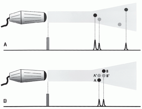
Lateral resolution varies throughout the field of imaging and is affected by several factors. The width or thickness of the interrogating beam, at a given depth, is the most important determinant. Ideally, the ultrasonic beam should be very narrow to provide a thin “slice” of the heart. Recall that the beam has finite width, even in the near field, and tends to diverge as it propagates. The importance of beam width stems from the fact that the system will display all targets within the path of the beam along a single line represented by the central axis of the beam. In other words, the echograph displays structures within the image as if the beam were infinitely narrow. Thus, lateral resolution diminishes as beam width (and depth) increases. The distribution of intensity across the beam profile will also affect lateral resolution. As illustrated in Figure 2.15, both strong and weak reflectors can be resolved within the central portion of the beam, where intensity is greatest. At the edge of the beam, however, only relatively strong reflectors may produce a signal. Furthermore, the true size and position of such objects may be distorted by the width of the beam, resulting in significant beam width artifacts. This is illustrated in Figure 2.15. This observation also explains the importance of overall system gain and its effect on lateral resolution. Gain is the amplitude, or the degree of amplification, of the received signal. When gain is low, weaker echoes from the edge of the beam may not be recorded and the beam appears relatively narrow. If system gain is increased, weaker and more peripheral targets are recorded and beam width appears greater. Thus, to enhance lateral resolution, a minimal amount of system gain should be employed. Figure 2.16 illustrates how changes in gain setting can drastically alter lateral resolution and anatomic information.
FIGURE 2.14. The different types of resolution. See text for details. PRF, pulse repetition frequency.
FIGURE 2.15. The interrelationship between beam intensity and acoustic impedance. The center of the beam has higher intensity compared with the edges. A: Whether an echo is produced, and with what amplitude it is recorded, depends on the relationship between intensity and acoustic impedance. Objects with higher impedance (black dots) produce stronger echoes and can, therefore, be detected even at the edges of the beam. Weaker echo-producing targets (gray dots) produce echoes only when they are located in the center of the beam. B: The effect of beam width on target location is shown. Objects A and B are nearly side by side with B slightly farther from the transducer. Because of the width of the beam, both objects are recorded simultaneously. The resulting echoes suggest that the two objects are directly behind each other (A′ and B′) rather than side by side.
A third component of resolution is called contrast resolution. Contrast resolution refers to the ability to distinguish and to display different shades of gray within the image. This is important both for the accurate identification of borders and for the ability to display texture or detail within the tissues. To convert the returning radio frequency (RF) information into a gray-scale image, pre- and postprocessing of the data are performed. These steps in image formation rely heavily on contrast resolution. From a practical standpoint, contrast resolution is necessary to differentiate tissue signals from background noise. Contrast resolution is also dependent on target size. A higher degree of contrast is needed to detect small structures compared with larger targets.
Temporal resolution, or frame rate, refers to the ability of the system to accurately track moving targets over time. It is dependent on the amount of time required to complete a scan, which in turn is related to the speed of ultrasound and the depth of the image as well as the number of lines of information within the image. Generally, the greater the number of frames per unit of time, the smoother and more aesthetically pleasing the realtime image. Factors that reduce frame rate, such as increasing depth of field, will diminish temporal resolution. This is particularly important for structures with relatively high velocity, such as valves. Temporal resolution is the main reason that M-mode echocardiography is still a useful clinical tool. With sampling rates of 1,000 to 2,000 images per second, temporal resolution of this modality is much higher than that of two-dimensional imaging.
Creating the Image
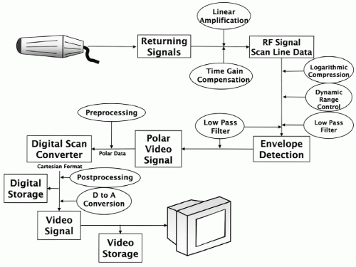
The instrument used to create an ultrasound image is called an echograph. It contains the electronics and circuitry needed to transmit, receive, amplify, filter, process, and display the ultrasound information. The essential components of the system are illustrated in Figure 2.17. As a first step, the returning energy is converted from sound waves to voltage signals. These are very low amplitude, high-frequency signals that must be amplified and, because they arrive slightly out of phase, realigned in time. In modern instrumentation, this realignment is accomplished using a digital beam former to allow proper summation and phasing of all the channels. Because the signals are still very high frequency at this point, the scan lines are referred to as RF data. The complexity of the information at this stage is in part due to the wide range of amplitudes and the inclusion of background noise. Logarithmic compression and filtering are performed to render the RF data more suitable for processing.
FIGURE 2.16. Parasternal long-axis images demonstrate the effect of gain on the appearance on the echocardiographic image. A: Gain is adjusted appropriately to allow recording of all relevant information. B: Too much gain is used, distorting the image, reducing resolution, and increasing noise.
The polar scan line data at this point consist of sinusoidal waves, and each ultrasound target is represented as a group of these high-frequency spikes. Each group of high-frequency RF data is consolidated into a single envelope through a curve-fitting process called envelope detection. The resulting signal is then referred to as the polar video signal. This is sometimes called R-theta, indicating that each point in a polar map can be defined by its distance (R) and angle (theta) from a reference point. The next very important step involves digital scan conversion and refers to the complex task of converting polar video data into a Cartesian or rectangular format. The image formed at this stage can be either stored in digital format or converted to analog data for videotape storage and display.
FIGURE 2.17. The components of an echograph. The various steps needed to create an image, beginning at the transducer and continuing to the display, are included. See text for details. RF, radio frequency.
Figure 2.18 displays these different forms of imaging data as energy is received and processed by the echograph. The energy created by excitation of the piezoelectric elements is an RF signal (Fig. 2.18A). As discussed in the previous section, for the signal to be in a form that can be displayed visually, it must be converted to a video signal. This is accomplished by outlining (envelope detection) the outer edge of the upper portion, or positive deflection, of the RF signal (Fig. 2.18B). Differentiation of the video signal effectively accentuates the leading edge of the echo (Fig. 2.18C), providing a brighter signal and improving the ability to differentiate closely spaced targets. This is sometimes referred to as A-mode, for amplitude, imaging. Finally, intensity modulation converts the height or amplitude of the signal to a corresponding brightness level for video display (Fig. 2.18D). This is often called B-mode, for brightness, imaging and forms the basis of both M-mode and two-dimensional imaging display. How these various signal formats are used to create a visual display is covered in greater detail in a later section.
Only gold members can continue reading. Log In or Register to continue