Since its inception, one of the primary goals of echocardiography has been to provide hemodynamic information. This was initially accomplished using M-mode and later two-dimensional imaging, which allowed measurement of dimensions that could be translated into volumetric data. The development of Doppler echocardiography now provides a more direct and quantitative technique from which to derive hemodynamic information. Currently, Doppler imaging, combined with two-dimensional imaging, is the preferred method for the noninvasive measurement of hemodynamics and, in many situations, has supplanted cardiac catheterization for this purpose. The accuracy of the Doppler technique for measuring blood velocity has been validated in numerous ways. Through its ability to quantify blood flow, measure pressure gradients, and estimate intracardiac pressures, the utility of Doppler-derived hemodynamic data is now well established.
Use of M-Mode and Two-Dimensional Echocardiography
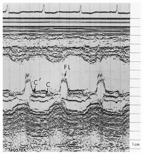
Since the early days of ultrasound, investigators have attempted to extract hemodynamic data from echocardiograms. Such approaches were indirect and qualitative, generally relying on the fact that physiologic changes in blood flow would have predictable effects on the motion of the walls and valves of the heart. One of the earliest applications arose from the recognition that right ventricular pressure and volume overload caused predictable changes in the motion of the interventricular septum. Unfortunately, little quantitative information could be derived from this observation. Thus, once Doppler techniques became available, a more direct quantitative measure of right ventricular pressure was possible, thereby supplanting these more indirect approaches. A more relevant observation involved the early closure of the mitral valve that occurred in patients with acute, severe aortic regurgitation (Fig. 9.1). Here, the high temporal resolution of the M-mode technique provided a unique approach for timing valvular events. Premature closure of the mitral valve indicated rapidly increasing left ventricular diastolic pressure and became a reliable, if indirect, marker of hemodynamically significant aortic regurgitation before the availability of more direct noninvasive techniques.
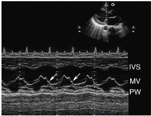
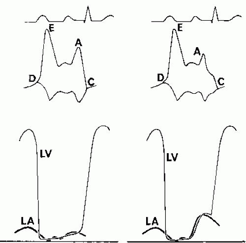
A similar example is the B bump of mitral valve closure. This is a particular motion of the mitral valve that occurs in late diastole as the valve drifts shut with increasing left ventricular pressure (Fig. 9.2). The normal rate of mitral valve closure after atrial systole is smooth and of brief duration. In patients with elevated left ventricular diastolic pressure, the associated increase in left atrial pressure results in an abnormal pattern of mitral valve closure. The onset of mitral valve closure is premature, and mitral valve closure is interrupted because the A point occurs earlier than usual, resulting in a notch between the A point and the C point. The prolongation of the closing phase of the mitral valve has been termed the B bump and has been associated with increased left ventricular end-diastolic (and left atrial) pressure (Fig. 9.3). Efforts to quantify left ventricular diastolic pressure using this finding have been unreliable. Although the sensitivity of the finding has been debated, the presence of a B bump is consistently associated with a left ventricular diastolic pressure at the time of atrial contraction of at least 20 mm Hg. The application of Doppler techniques to the study of left atrial pressure eventually overshadowed the importance of this finding.
FIGURE 9.1. A mitral valve M-mode echocardiogram from a patient with acute aortic regurgitation. Note partial valve closure (C′) in middiastole, significantly earlier than normal. The valve does not reopen with atrial systole and then closes completely with the onset of ventricular contraction (C). Fine fluttering (FL) of the mitral valve is due to the aortic regurgitant jet.
FIGURE 9.2. A mitral valve echocardiogram demonstrating a B bump (arrows). See text for details. IVS, interventricular septum; MV, mitral valve; PW, posterior left ventricular wall.
FIGURE 9.3. A schematic demonstrates how the mitral valve echocardiogram reflects changes in left ventricular diastolic pressure. The normal relationship between mitral leaflet motion and intracardiac pressure changes is shown on the left. The genesis of the B bump reflects elevated late diastolic left atrial pressure. See text for details.
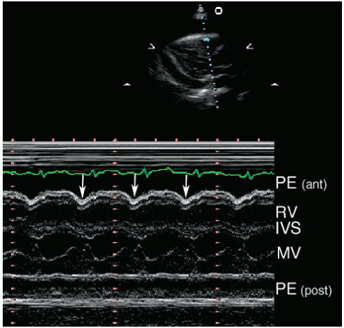
Other M-mode echocardiographic signs of altered hemodynamics also have stood the test of time. Systolic anterior motion of the mitral valve is an important finding in patients with hypertrophic cardiomyopathy and may indicate dynamic outflow tract obstruction. This is demonstrated using either M-mode or two-dimensional techniques. In these patients, partial closure of the aortic valve during mid and late systole, as seen on M-mode echocardiography, is a reliable indicator of significant outflow tract obstruction. Again, however, quantification of the gradient is not possible. One of the most useful echocardiographic indicators of hemodynamic significance is the early diastolic collapse of the right ventricular free wall that occurs when intrapericardial pressure increases in the clinical setting of tamponade (Fig. 9.4). This is discussed in detail in Chapter 10.
FIGURE 9.4. An M-mode echocardiogram from a patient with pericardial tamponade. The arrows indicate early diastolic collapse of the right ventricular free wall. The echo-free space above the right ventricular free wall represents pericardial fluid, which can also be seen posterior to the left ventricle. IVS, interventricular septum; MV, mitral valve; PE, pericardial effusion.
Table 9.1 M-Mode and Two-Dimensional Echocardiographic Findings of Altered Hemodynamics
Finding
Hemodynamic Significance
M-mode
Early closure of the mitral valve
Acute, severe aortic regurgitation
Increased mitral valve E point-septal separation
Reduced LV ejection fraction
Delayed closure of the mitral valve (B bump)
Elevated LV end-diastolic pressure
RV free-wall early diastolic collapse
Pericardial tamponade
Midsystolic notching of the aortic valve
Dynamic subaortic outflow tract obstruction
Diastolic mitral valve fluttering
Aortic regurgitation
Midsystolic notching of the pulmonary valve
Pulmonary hypertension
Rounding of the opening/closing points of a disk-type prosthetic valve
Mechanical restriction to disc motion
Systolic anterior motion of the mitral valve
Dynamic subaortic outflow track obstruction
Early systolic downward motion (beaking) of the IVS
LBBB
Gradual closure of the aortic valve
Reduced left ventricular stroke volume
Absent pulmonary valve A wave
Pulmonary hypertension
Two dimensional
Diastolic flattening of the IVS
RV volume overload
Systolic flattening of the IVS
RV pressure overload (elevated RVSP)
Dilated IVC with abnormal respiratory variation
Elevated RA pressure
Exaggerated IVS bounce, with respiratory variation
Constriction
IVC, inferior vena cava; IVS, interventricular septum; LBBB, left bundle branch block; LV, left ventricle; RA, right atrial; RV, right ventricular; RVSP, right ventricular systolic pressure.
A partial listing of M-mode and two-dimensional echocardiographic findings indicating abnormal hemodynamics is provided in Table 9.1. Although most of these findings have been replaced by more quantitative and direct measurements using the Doppler techniques, they continue to provide useful confirmatory evidence in selected patients.
Quantifying Blood Flow
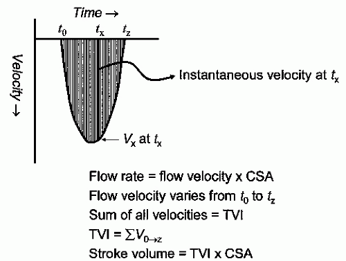
Doppler echocardiography is able to measure blood flow through its ability to quantify blood velocity. We know that the rate of flow through an orifice is equal to the product of flow velocity and cross-sectional area. Because cross-sectional area can be measured with M-mode or two-dimensional imaging and flow velocity can be determined directly with Doppler imaging, the technique provides a noninvasive measure of flow. If flow were constant (i.e., had a fixed velocity), it would be a simple matter to determine velocity at any point in time and solve the equation accordingly. In the cardiovascular system, however, flow is pulsatile and therefore individual velocities during the ejection phase must be sampled and then integrated to measure flow volume. This sum of velocities is called the time velocity integral (TVI) and is equal to the area enclosed by the Doppler velocity profile during one ejection period. This essential concept is illustrated in Figure 9.5. Integrating the area under the velocity curve is simply measuring the velocities at each point in time and summing all these velocities. It should be noted that when velocity is integrated over time, the units that result from this operation are a measure of distance (in centimeters), hence the term stroke distance, which is the linear distance that the blood travels during one flow period. When TVI and the corresponding cross-sectional area (in centimeters squared) are measured at the same point, such as through one of the four cardiac valves, their product equals stroke volume (in centimeters cubed or milliliters), which is the volume of blood ejected by the heart with each contraction (assuming no valvular regurgitation or cardiac shunt).
FIGURE 9.5. A schematic demonstrates the concept of flow quantification using the Doppler technique. Doppler records instantaneous velocity throughout the cardiac cycle. The area under the Doppler velocity curve represents the time velocity integral (TVI). This is the sum of all the individual instantaneous velocities throughout the ejection period. See text for details. CSA, cross-sectional area.
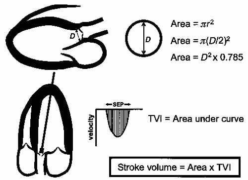
These principles are illustrated in Figure 9.6, which demonstrates how these concepts can be applied to aortic flow to measure stroke volume. Recall from the Doppler equation the importance of the angle θ, that is, the angle between the ultrasound beam and blood flow direction. Because the cosine function varies between 0 and 1 and appears in the numerator of the Doppler equation, errors in θ will have a predictable effect on measured velocities. For example, if θ is between 0 and 20°, the cosine of θ will range between 1.0 and 0.92, leading to a slight underestimation of true velocity. As θ increases to more than 20°, the cosine decreases rapidly and the degree of velocity underestimation increases quickly. Hence, aligning the ultrasound beam as close as possible to the direction of flow is critical if true velocity is to be measured. Equally important, misalignment between the ultrasound beam and flow can result only in underestimation of velocity, never overestimation.
FIGURE 9.6. The method for quantifying stroke volume. Two measurements are required: area and time velocity integral. See text for details. D, diameter; SEP, systolic ejection period; TVI, time velocity integral.
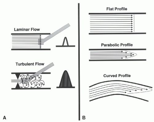
FIGURE 9.7. A: The differences between laminar and turbulent flow are demonstrated using pulsed Doppler. Laminar flow is associated with a lower velocity and a thinner flow envelope. B: Various flow profiles are provided. See text for details.
Another factor that will affect the accuracy of the Doppler equation is the pattern of blood flow in which velocity is being measured. Normal flow in the heart and great vessels is laminar, meaning that the fluid is traveling at approximately the same velocity and in the same general direction. If a sample volume is placed within such a flow pattern, the Doppler will record a clean signal of uniform velocity. Flow becomes increasingly disturbed or turbulent (i.e., less laminar) as the velocity increases or the cross-sectional area changes (Fig. 9.7A). Viscosity also affects the flow profile. At the edge of the flow pattern, near the vessel wall, flow tends to be slower and more turbulent. The highest velocities and most laminar flow generally occur at the center of the profile. This spatial distribution of velocities across the three-dimensional flow is called the flow velocity profile. In a large, straight vessel, with laminar flow, it tends to be flat (Fig. 9.7B), whereas in smaller curved vessels, the profile has a parabolic shape. Velocity will be higher at the center and lower at the margins. Flow patterns through curved vessels, such as the aortic arch, are more complex. Here the distribution of velocities depends on the size of the vessel, the flow profile entering the curve, and the presence and location of branch vessels. If the sample volume is placed within such a flow pattern, the recorded velocity will vary, depending on the exact location.
Fortunately, flow passing through a normal heart valve or the proximal great vessels tends to be laminar with a flat profile and is therefore suitable for quantitative analysis. Because it is easier to determine the average flow velocity with a flat versus a parabolic blood profile, it is not surprising that efforts to measure blood flow attempt to use larger orifices and flow that are close to the origin of vessels. Also note that physiologic blood flow is never perfectly uniform. That is, at any point in time, a distribution of velocities occurs, resulting in a broadening of the Doppler signal. The greater the range of velocities is at any point in time, the broader is the Doppler signal. The darker line through the center of the distribution represents the modal frequency, that is, the velocity at which the largest number of blood cells are traveling (Fig. 9.8). Theoretically, this is the velocity that should be used to determine the TVI. In practice, however, it is common to trace the outer edge of the densest portion of the envelope, and studies have indicated that both techniques provide a reasonably accurate measurement of blood flow. Multiple cycles (usually three to five) should be traced and averaged to minimize error. In patients with atrial fibrillation, between 5 and 10 beats should be analyzed.
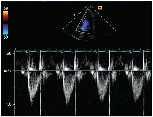
FIGURE 9.8. An example of laminar flow through the aortic valve recorded from the apical view with pulsed Doppler imaging. The vertical velocity spike at end-systole indicates aortic valve closure.
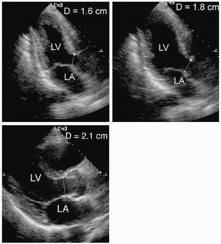
FIGURE 9.9. To measure the cross-sectional area of the left ventricular outflow tract, the diameter (D) must be measured carefully. The three examples demonstrate three different values for D obtained from the same patient. In most cases, the correct dimension is the largest, indicating the true diameter.
An important potential source of error in the blood flow measurement is the determination of cross-sectional area. It is essential to remember that cross-sectional area must be measured at the same point in space where the Doppler signal is sampled. For example, if blood flow is measured through the aortic valve, both the Doppler signal and the cross-sectional area must be measured at the same level. If the Doppler sample volume is placed at the level of the aortic annulus, then the cross-sectional area of the aortic annulus must be determined. The cross-sectional area can be measured in systole using either M-mode or two-dimensional imaging. In Figure 9.9, three slightly different measurements of the outflow tract diameter are obtained. In most cases, the largest dimension should be used because it most likely corresponds to the true diameter. Another approach to this problem would be to directly measure the cross-sectional area by planimetry of a short-axis image of the orifice. In practice, however, it is common to determine the diameter of the orifice, assume a circular shape, and calculate area using the formula
Because r = ½D, and D is what is actually measured, this can be simplified and expressed as
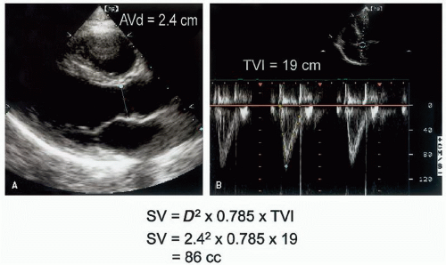
FIGURE 9.10. An example of stroke volume calculation. A: The cross-sectional area of the outflow tract (AVd) is measured. B: The time velocity integral of aortic flow is determined by planimetry. The calculation for stroke volume (SV) is shown. TVI, time velocity integral.
Thus, the Doppler equation for stroke volume becomes
Considering this equation, it is obvious that any error in the measurement of the diameter of the orifice is “squared” and thus contributes greatly to errors in the final determination. For this reason, particular care must be taken to ensure accurate determination of orifice diameter. Multiple measurements should be performed. Generally, the largest dimension is used because it most likely represents the true diameter and smaller measurements represent tangential cuts through the circular outflow tract. The importance of accurately measuring the outflow tract diameter is illustrated in the following example. Assume that the “true” diameter is 2.0 cm and the TVI is 20 cm. This would yield a stroke volume of 63 mL. Underestimation of the diameter by just 10% would have the following effect on stroke volume calculation:
Stroke volume = 0.785 × (1.8 cm)2 × 20 = 51 mL
Thus, a 2-mm (or 10%) underestimation in diameter would lead to a 19% underestimation (51 mL instead of 63 mL) in stroke volume.
Despite these potential sources of error, several investigators have demonstrated the accuracy of this approach for measuring blood flow in a variety of clinical situations. When performed carefully, this noninvasive technique has proven to be an accurate and reproducible way to quantify blood flow within the cardiovascular system. An example of stroke volume calculation from the aortic flow measurement is provided in Figure 9.10.
Clinical Application of Blood Flow Measurement
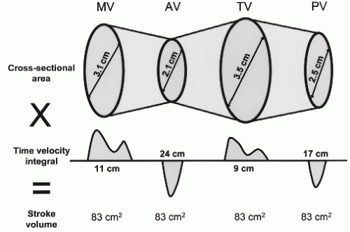
The Doppler approach to measuring blood flow is a general formula that can be applied anywhere that blood passes through an orifice of fixed and measurable dimensions. Thus, it is possible to measure blood flow across all four valves of the heart and in the great vessels. To do so requires pulsed Doppler sampling of flow velocity at a location where cross-sectional area also can be measured. Figure 9.11 illustrates how stroke volume can be measured through each of the four valves. In the absence of valvular regurgitation or intracardiac shunt, flow through all four valves should be equal. The diagram demonstrates how cross-sectional area and TVI vary inversely for the different valves, but the product (cross-sectional area × TVI) is equal at each location. Of course, each site presents its unique set of challenges, and in any given patient, the measurement may or may not be feasible. Accuracy and reproducibility will improve with practice. Thus, performing flow calculation on a routine basis can be expected to increase one’s confidence in the results when clinical questions arise.
Although flow can theoretically be measured at any site, in practice, it is customary to measure blood flow through the aortic valve. The Doppler recording is performed using either the apical five-chamber or the apical long-axis view and the sample volume is positioned at the level of the aortic annulus, approximately 3 to 5 mm proximal to the valve (Fig. 9.10). At that location, it is usual to record the closing “click” of the aortic valve at end-systole. If the opening click is present in the Doppler recording, the sample volume should be withdrawn slightly into the outflow tract. Cross-sectional area is measured by recording the parasternal long-axis view and determining the diameter of the aortic annulus in systole, assuming a circular shape. Because annular size does not change much over the cardiac cycle, the precise timing of the diameter measurement is not critical. Alternatively, the annulus can be viewed from the shortaxis projection and the area measured directly via planimetry. This is theoretically more precise but practically more difficult.
FIGURE 9.11. This schematic demonstrates the principle of conservation of mass. In the absence of valvular regurgitation or intracardiac shunts, the stroke volume through each of the four valves should be equal. See text for details. AV, aortic valve; MV, mitral valve; PV, pulmonic valve; TV, tricuspid valve.
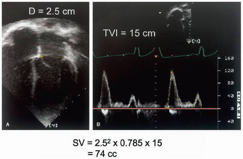
FIGURE 9.12. An example of calculating stroke volume (SV) through the mitral valve. A: The cross-sectional area of the mitral annulus is determined. B: Flow velocity at that level is measured using pulsed Doppler imaging. See text for details. TVI, time velocity integral.
Pulmonary valve flow can be recorded using a similar approach. The sample volume is positioned at the level of the pulmonary valve, usually from the basal short-axis view. Alternatively, especially in children, the subcostal short-axis view can be used. The cross-sectional area is measured as the diameter of the outflow tract at the level of the annulus. An accurate measurement of this diameter is often difficult in adults because of the challenges of visualizing the lateral border of the right ventricular outflow tract. It is commonly performed in children, however, to quantify right ventricular stroke volume. This can then be compared with stroke volume in the left side of the heart to assess intracardiac shunts and valvular regurgitation. This application is covered later in this section.
Quantitating stroke volume across the mitral valve creates additional challenges. Mitral flow velocity is easily recorded from apical views and consists of two phases: an early diastolic wave (E) and a second wave associated with atrial systole (A). Several studies have demonstrated that Doppler mitral velocity can be used to quantify stroke volume provided that the crosssectional area of the mitral valve orifice can be determined. This can be performed using a short-axis view to planimeter its cross-sectional area. Next, an M-mode or two-dimensional echocardiographic recording of the mitral valve is used to determine the mitral orifice diameter throughout diastole. From this, the mean mitral diameter is calculated and applied to the Doppler equation. A simplified and more practical approach uses the diameter of the mitral annulus as measured from the apical views as a surrogate for cross-sectional area (Fig. 9.12). The measurement should be performed from the four-chamber view in early diastole. Then, assuming a circular shape, the area is estimated by Equation 9.1, which is A = πr2. Alternatively, a second diameter can be measured from the apical two-chamber view and a mean value for cross-sectional area can be obtained. Mitral inflow velocity is then recorded at the level of the annulus, and the TVI is determined by planimetry (Fig. 9.13). The accuracy of quantifying mitral stroke volume is debatable. Recording a clean velocity profile at the annular level (compared with the mitral leaflet tips) can be challenging. It is also more difficult to accurately measure cross-sectional area at the mitral annulus compared with the aortic annulus. For all these reasons, quantifying blood flow across the mitral and tricuspid valves is more cumbersome compared with the aortic and pulmonary valves and is performed rarely in clinical practice.
This technique for determining volumetric flow has several practical applications. The noninvasive measurement of stroke volume has obvious value, both as an absolute number and as a relative change. Stroke volume is a fundamental measure of global left ventricular systolic performance and can be readily converted to cardiac output by multiplying by heart rate. In critically ill patients, relative changes in stroke volume may indicate improvement or deterioration or may reflect a response to an intervention. In this case, it is the relative change that matters. If cross-sectional area is assumed to remain constant, changes in the TVI will reflect changes in stroke volume. This has the advantage of avoiding the potential errors that can be introduced when measuring cross-sectional area. By following changes in TVI, relatively subtle alterations in cardiac performance can be tracked.
In patients with valvular regurgitation, differences in stroke volume across different valves provide a quantitative assessment of severity. This is illustrated schematically in Figure 9.14. In the absence of regurgitation, stroke volume across all four valves should be equal. In the presence of aortic regurgitation, for example, the difference between aortic flow and mitral flow represents the aortic regurgitant volume as shown in the following formula:
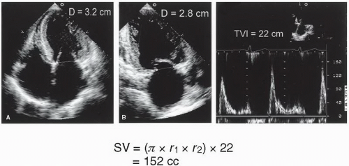
FIGURE 9.13. An alternative approach to quantification of flow through the mitral valve assumes an elliptical shape of the mitral annulus. The diameter is measured from the four-chamber (A) and two-chamber (B) views. The Doppler recording of mitral inflow is shown on the right. The equation for the area of an ellipse is A = π × r1 × r2. The stroke volume (SV) calculation is shown. TVI, time velocity integral.
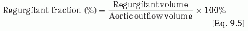
Regurgitant fraction in aortic regurgitation can also be calculated as
This type of calculation can be performed for any valve of the heart (Fig. 9.15). It assumes that the valve used as the standard for flow is not regurgitant and that a similar degree of accuracy can be achieved at each location. In addition, the calculation is complicated by the presence of valve stenosis.
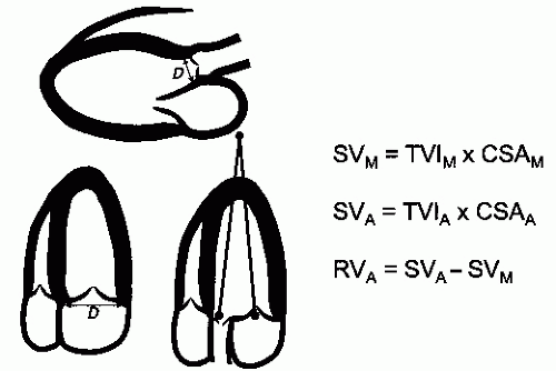
FIGURE 9.14. Differences in stroke volume (SV) across the aortic and mitral valves may reflect regurgitation at one of these sites. In this schematic from a patient with aortic regurgitation, regurgitant volume (RVA) is simply the difference between the aortic stroke volume and the mitral stroke volume. CSA, cross-sectional area; D, diameter; TVI, time velocity integral. See text for details.
A final application of this principle is the quantitation of intracardiac shunts. Determining the pulmonary-to-systemic flow ratio, or Qp:Qs, is the principal way to quantitate the size of the shunt (Fig. 9.16). In most cases, the shunt ratio is determined by calculating pulmonary stroke volume and comparing it with aortic stroke volume. The difference equals the net shunt volume in the absence of semilunar valve stenosis or regurgitation. This approach has been used in pediatric echocardiography with success and has been validated against invasive standards.
In summary, calculation of volumetric flow is possible and has been validated in a variety of clinical situations. The formulas are based on sound physiologic principles and, under optimal circumstances, provide an accurate means for quantifying flow. Measurement errors can cause significant mistakes that may or may not be apparent at the time of the calculations. As a consequence, a small and sometimes unrecognized error in measurement can lead to an unacceptable error in the final result. For example, if aortic and mitral stroke volumes are derived to calculate regurgitant volume and if each primary calculation is off by 10%, the following scenario is possible. Assume that the correct aortic stroke volume is 90 mL and the mitral stroke volume is 60 mL, yielding a regurgitant volume of 30 mL and a regurgitant fraction of 33%. If the aortic stroke volume is high by 10% (99 mL) and the mitral stroke volume is low by the same degree (54 mL), the derived regurgitant volume is now 45 mL and the regurgitant fraction is 45%, a significant difference. To minimize the likelihood of errors, it is essential to do such calculations routinely rather than just on rare occasions. Be aware of the potential sources of error and know when image quality precludes reliable measurements.
Only gold members can continue reading. Log In or Register to continue