14
Aortic Valve Anatomy and Embryology
The aortic valve (AV), located at the base of the aorta, comprises three semilunar cusps and functions to allow unidirectional blood flow from the left ventricle into the systemic circulation. AV closure prevents blood from flowing backward into the left ventricular outflow tract (LVOT) and left ventricle. The AV’s three cusps are named for their relationships to the coronary ostia (right, left, and noncoronary cusps) and have three corresponding sinuses of Valsalva (right, left, and noncoronary sinuses). The AV ascends at the level of the commissures between the cusps and descends toward (but not into) the LVOT at the base or nadir of the cusps.1–3 The sinuses of Valsalva become continuous with the left ventricle at the lower margin of the aortic root and meet the ascending aorta at the upper margin. 4 The upper margin of the sinuses (where they meet the tubular portion of the aorta) is the sinotubular junction. The aortic wall and LVOT have both muscular and fibrous components. The LVOT consists of a muscular membranous septal component and a fibrous posterior quadrant that is continuous with the fibrous skeleton of the heart. The base of the anterior leaflet of the mitral valve has a fibrous connection to the left and noncoronary cusps and constitutes the aortomitral continuity. The AV lacks a discrete annulus. The attachments of the AV cusps to the aorta and left ventricle are curvilinear. The three cusps meet centrally during diastole at the nodule of Arantius. 3
The AV and its supporting sinuses develop within a turret of cardiac muscle.5,6 The initial muscular walls of the intrapericardial trunks become transformed to arterial structures with separation of the adjacent aorta and pulmonary trunks. The sinus walls of the roots are also formed of arterial tissues. 7 The aortic and pulmonary valves are quite similar histologically in the fetus. Histologic differences develop after birth between the aortic and pulmonary valves related to molecular stability and cross-linking of collagen. After birth, the neonatal AV collagen becomes more unstable owing to the increase in transvalvular pressure compared to the low transvalvular gradients exerted on the pulmonic valve. Changes in the molecular stability and cross-linking of collagen of the AV during the transition from fetal to neonatal circulation appear to be due to increased transvascular pressure gradients. 8 In the adult, the AV cusps become thicker and are composed of denser collagen fibers with compartmentalization of vascular interstitial cells, compaction, and stratification of the extracellular matrix into a trilaminar structure.8–10 The pulmonic valve remains thin with less collagen compared to the AV. 8 These differences in the semilunar valves can be seen with both visual inspection and transesophageal echocardiography (TEE). The applicability of these insights become useful in both achieving a better understanding of the anatomy and embryology of the AV and in production and tissue engineering of prosthetic heart valve replacements for both the pulmonic and aortic positions. 9 The other application of these structural differences in the semilunar valves is in the surgical explant and transfer of the pulmonary valve to the aortic position during the Ross procedure. 11 The central position of the AV relative to the atria, pulmonary trunk, and ventricles render these adjacent structures susceptible to involvement (e.g., fistula) in the setting of endocarditis and abscess. 12
In a small percentage of individuals, excessive fusion between cushions or ridges of the aortic cusp can produce a septum in the developing outflow tract. 7 Bicuspid AVs develop when excessive fusion of ridges results in conjoined leaflets. This most often occurs between the leaflets arising from the sinuses of the right and left coronary cusps. A less common mechanism in the formation of a bicuspid AV is a relative paucity of endothelial nitric oxide synthase, which may result in a phenotype in which the conjoined leaflets represent fusion of the noncoronary and right coronary cusps.12,13 In either case, the presence of a bicuspid AV predisposes to both aortic insufficiency and early calcification and stenosis; this is one of the most common etiologies of aortic pathology in patients presenting for AV surgery.
 Transesophageal Echocardiographic Views for Aortic Valve Assessment
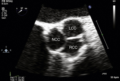
Midesophageal Aortic Valve Short-Axis View
The midesophageal (ME) AV short-axis (SAX) view ( Fig. 14-1 and  Video 14-1) is generated with the tip of the TEE probe in the esophagus and the ultrasound transducer rotated to approximately 35 to 50 degrees. The images generate an en face view of the AV akin to the view of the surgeon when peering through an aortotomy incision. The valve is inspected by echocardiography in diastole (closed) and systole (open). In normal valves, the cusps are thin and freely mobile. The systolic orifice area can be measured by planimetry (or calculated via the continuity equation using other views). “Normal” individuals may have a tiny jet of trace aortic regurgitation (AR), often located in the center of the AV. In the presence of AR, the SAX view is particularly useful in defining the locus of the regurgitant orifice. Ostia of the left main and right coronary arteries are easily detected emanating from the corresponding coronary sinuses. Slight withdrawal of the TEE probe demonstrates the proximal ascending aorta. Advancement of the probe depicts the LVOT.
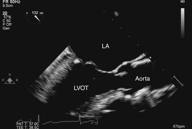
Midesophageal Aortic Valve Long-Axis View
The ME-AV long-axis (LAX) view ( Fig. 14-2 and Video 14-2  ) is produced by rotating the transducer to approximately 120 to 150 degrees. Blood flow is mostly perpendicular to the ultrasound beam. The LVOT, valve cusps, sinuses, sinotubular junction, and ascending aorta are seen in a single image. The mobile cusps of the AV produce a zone of coaptation and effacement during diastole that spans several millimeters. The cusps separate widely during systole in normal patients (where the AV area is ≈ 2.6-3.5 cm2). The sinuses of Valsalva are seen as symmetric outpouchings that form an aortic root bulb that joins the ascending aorta at the sinotubular junction. The AV LAX view is suitable for assessing the grade of AR with color Doppler. Application of color Doppler in the normal AV demonstrates no transvalvular flow during diastole but laminar flow during systole.
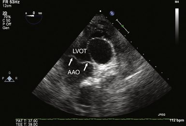
Deep Transgastric Long-Axis View of Aortic Valve
The deep transgastric (TG) LAX view of the AV ( Fig. 14-3 and Video 14-3) is obtained by insertion and anteflexion of the probe from the TG SAX imaging plane and can be difficult to attain without significant flexion of the probe in the stomach. However, the TG view can often align the transvalvular flow parallel to the ultrasound beam, rendering TEE reliable in detecting and quantifying transvalvular blood flow velocities. It is the preferred view for spectral Doppler measurements of flow velocities to generate estimates of AV gradients and spectral displays of regurgitant jets.
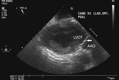
Transgastric Long-Axis View of Aortic Valve
The TG LAX view of the AV ( Fig. 14-4) is obtained at an angle of 110 to 135 degrees from the TG SAX view of the left ventricle. Like the deep TG view, it allows for parallel alignment of the ultrasound beam with transaortic flow, making it an excellent choice for spectral Doppler interrogation of the AV. In addition, ME views of the AV may be obscured by echo shadowing in patients with significant mitral annular calcification or in patients with prosthetic mitral valves and mitral annuloplasty rings. In these scenarios, both deep TG and TG LAX views often allow imaging of the AV without overlying shadowing.
 Aortic Stenosis
Anatomic Imaging in Aortic Stenosis
A thorough two-dimensional (2D) echocardiographic examination of the AV usually yields the first evidence of stenosis. Increased valve echogenicity secondary to calcifications is typically present in patients with aortic stenosis (see  Video 14-4). Although increased echogenicity can be due solely to leaflet sclerosis, the calcifications seen in true aortic stenosis are associated with leaflet thickening and a reduction in valve opening. The pattern of calcification can also provide insight into the underlying etiology of the valve stenosis ( Fig. 14-5). In senile calcific degeneration of tricuspid AVs, the bodies of the leaflets are most affected. In rheumatic stenosis, commissural fusion may be the most outstanding feature. With advanced rheumatic or bicuspid aortic stenosis, the degree of calcification may be so great that echocardiographic distinction between entities is impossible. A full anatomic evaluation should also include an assessment of both the subvalvular ( Fig. 14-6) and supravalvular areas to rule out nonvalvular stenosis. 14
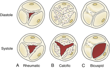
Figure 14-5 Morphology of valve calcification and etiology of stenosis. A, Rheumatic disease with commissural fusion. B, Senile calcific degeneration of leaflet bodies. C, Bicuspid valve with fused raphe. (Adapted from Baumgartner H, Hung J, Bermejo J, et al. Echocardiographic assessment of valve stenosis: EAE/ASE recommendations for clinical practice. J Am Soc Echocardiogr. 2009;22:1-23.)
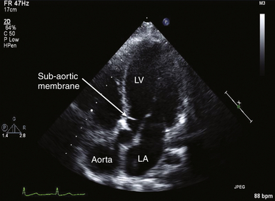
Figure 14-6 Subaortic membrane. In this deep transgastric long-axis image, membrane is seen within left ventricular outflow tract, creating stenosis proximal to aortic valve. LA, Left atrium; LV, left ventricle.
In addition to qualitative evaluation, 2D imaging can be used to quantify the severity of the stenosis. The simplest technique for quantification is to measure leaflet separation in long axis. This is best accomplished in the ME-AV LAX view ( Fig. 14-7), although the deep TG LAX view can yield acceptable results as well. When the separation is greater than 15 mm, significant obstruction can be reliably excluded. 15 When using this quantification technique, it is important to align the 2D image in the center of the valve; a sector cut closer to a commissure may lead to overestimation of the degree of stenosis. In the ME-AV LAX view, a 2D-guided M-mode measurement of leaflet separation can also be used. Given the more complex leaflet orientation seen in congenital valve stenosis, use of leaflet separation to estimate the severity of stenosis may be less accurate. 15
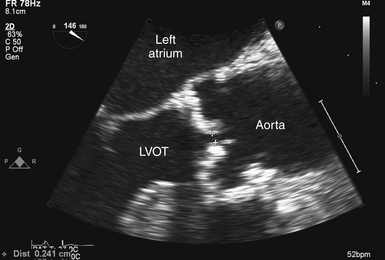
Figure 14-7 Measurement of leaflet separation in trileaflet valve. Transesophageal echocardiographic image obtained from zoomed midesophageal aortic valve long axis. Effort is made to image through center of aortic valve. NOTE: leaflet edges are parallel to each other and within aortic root. LVOT, Left ventricular outflow tract.
Direct valve orifice area measurements can be obtained using valve planimetry in the ME-AV SAX view. Planimetry is performed by tracing the area of the valve orifice using echocardiographic software packages ( Fig. 14-8). To increase accuracy, it is important to trace the valve orifice at the level of the leaflet tips, because measurements obtained near the base of the leaflets may overestimate valve area and underestimate the severity of stenosis. Planimetry is usually straightforward in patients without significant leaflet calcification ( Fig. 14-9), but in those with significant calcification, the ability to clearly visualize and define the true valve orifice may be impeded. This limitation will also apply if the valve has a complex 3D orientation leading to a nonplanar orifice ( Fig. 14-10) and may be even more relevant in congenital lesions ( Fig. 14-11). 3
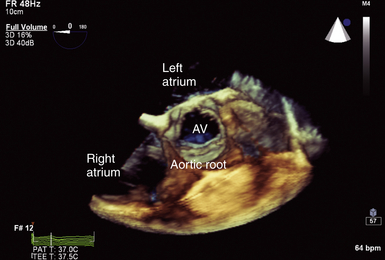
Figure 14-8 Full-volume three-dimensional image focused on aortic root with normal trileaflet aortic valve (AV) seen in center of image. Note cylindrical nature of this normal valve orifice, which facilitates ability to measure leaflet separation or valve area planimetry.
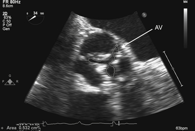
Figure 14-9 Planimetry of aortic valve (AV): zoomed midesophageal AV short-axis view. AV is seen in its short axis in center of image, with its area traced. To optimize accuracy, multiple measurements should be made to ensure smallest planar area is measured.
Figure 14-10 In comparison to Figure 14-8, note the complex three-dimensional (3D) height of this severely stenotic aortic valve in A. This complexity is not readily apparent in corresponding two-dimensional (2D) image in B. This inability to appreciate 3D orientation limits accuracy when performing planimetry of 2D images.
Doppler-Derived Quantification of Aortic Stenosis
To properly interpret Doppler-derived measurements, an understanding of the nature of fluid dynamics through a stenotic orifice is important. Acceleration of blood flow during ventricular systole into a naturally occurring tapered ventricular outflow tract (LVOT) creates a uniform velocity flow profile throughout the entire outflow tract. As blood from the LVOT approaches a stenotic AV, flow accelerates and converges just proximal to the stenosis ( Figs. 14-12 and 14-13 and  Video 14-5). This acceleration continues as the jet crosses the stenosis. The jet reaches its narrowest width and highest velocity just downstream from the stenotic valve. This point is called the vena contracta ( Fig. 14-14; also see Fig 14-13).
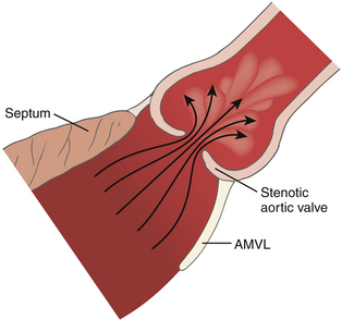
Figure 14-12 Flow through a stenotic orifice. AMVL, Anterior mitral valve leaflet. (From Otto CM, ed. Textbook of Clinical Echocardiography. Philadelphia: WB Saunders; 2000.)
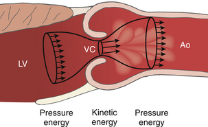
Figure 14-13 Recovery of pressure distal to a stenosis. Distal to the vena contracta (VC), the flow stream expands and kinetic energy is converted back to pressure energy in the aorta (Ao) minus any irrecoverable energy losses due to frictional and heat losses. LV, Left ventricle. (Adapted from Bach DS. Echo/Doppler evaluation of hemodynamics after aortic valve replacement: principles of interrogation and evaluation of high gradients. JACC Cardiovasc Imaging. 2010;3:296-304.)
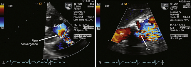
Figure 14-14 A, Deep transgastric long-axis (LAX) view with color flow Doppler (CFD) demonstrating prestenotic flow convergence in patient with aortic stenosis. B, Zoomed midesophageal aortic valve LAX view with CFD demonstrating vena contracta (VC) at level of stenotic valve. LVOT, Left ventricular outflow tract.
Distal to the vena contracta, flow expands and the jet velocity begins to fall. The pressure in the aorta distal to the vena contracta rises as blood flow velocity decreases, eventually reaching a level corresponding to the overall “pressure drop” across the stenosis. The distance the high-velocity jet travels into the ascending aorta will also be dependent on the angle of blood flow.16,17 Blood flow adjacent to the high-velocity jet is typically disturbed and characterized by disorganized movement with varying velocities (see Fig. 14-12). 15 The degree of flow disturbance is most related to the severity of the stenosis but will also be affected by the geometry of both the valve and ascending aorta. 18
Use of the Bernoulli Equation
Because the pressure gradient across a stenotic valve is directly related to the degree of valve narrowing, calculation of peak and mean gradients are frequently used to quantify the degree of aortic stenosis. Although pressure gradients cannot be measured directly via echocardiography, they can be derived from flow velocities obtainable using spectral Doppler. As described in Chapter 4, pressure gradients are related to jet velocity through the use of the modified Bernoulli equation:
Thus, by simply measuring the maximum velocity across the valve, the peak pressure gradient can be easily and reliably calculated.19,20 The mean gradient can be determined by tracing the obtained velocity curve and using the instrument software package to average the instantaneous velocities over the entire ejection period ( Fig. 14-15).
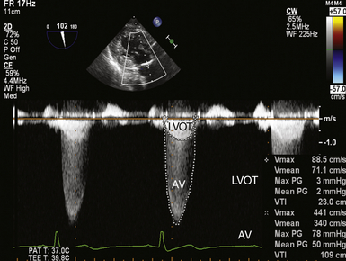
Figure 14-15 Double envelope technique; image obtained in deep transgastric long-axis view with continuous wave cursor placed crossing aortic valve (AV). Once obtained, the lower-velocity but denser left ventricular outflow tract (LVOT) curve is traced, as is the larger-velocity transvalvular curve, producing peak and mean gradients and velocity-time integrals (VTIs) for both velocity curves.
The velocity profile in aortic stenosis is best obtained from TG imaging planes that allow for parallel alignment of the Doppler beam with transaortic flow. Because the velocity of blood flow in clinically significant aortic stenosis is usually elevated, continuous wave Doppler (CWD) should be used to avoid pulsed wave Doppler (PWD) aliasing. Use of the simplified Bernoulli equation has been well validated, but there are some potential pitfalls. Most critically, the Doppler beam must be aligned parallel to the transaortic flow, because angles of intercept greater than 30 degrees can produce significant error and underestimation of the severity of stenosis. 14 To this end, it is helpful to utilize color flow Doppler (CFD) to visualize the jet crossing the valve (see Fig. 14-14, A) to help align the spectral Doppler beam. However, it is important to remember that even if the jet and Doppler beam appear well aligned in the visualized tomographic plane, the eccentric nature of many jets makes it impossible to know with certainty whether the alignment is optimized in the elevational plane.
For the most accurate results, multiple recordings should be made and ideally in more than one echocardiographic view, searching for the largest velocity obtainable. The recorded Doppler envelope with the highest velocity and a well-defined smooth velocity curve should then be used to derive gradients. In patients with significant stenosis, the ejection period is longer, creating a more rounded curve rather than more triangular. Patients with irregular rhythms will require additional effort to select representative tracings while avoiding use of post-PVC (premature ventricular contraction) beats. 14
When trying to explain these discrepancies, it is important to remember that the simplified Bernoulli equation eliminates LVOT velocity from the pressure gradient calculation. In patients with elevated LVOT velocities (>1.5 m/s), including those with AR, the proximal velocity term in the simplified Bernoulli equation cannot be ignored. Similarly, when the maximum transaortic velocity is less than 3 m/s, the LVOT velocity should also be reintroduced to provide for more accurate results. 14
Continuity Equation
Because of the major influence trans-AV flow exerts on pressure gradients, use of the continuity equation to calculate AV area has become an important tool for quantification of stenosis severity. As described in Chapter 4, the continuity equation is based on the concept of the continuity of flow or mass. In the case of the AV, stroke volume through the LVOT should remain equal to that of stroke volume through the AV.

Measurement of LVOT diameter is best obtained in the ME-AV LAX view and should be measured leading edge to leading edge, just proximal to the AV and as parallel to the valve plane as possible ( Fig. 14-16). Because the diameter is squared in calculating LVOT area, small variations in its measurement can lead to substantial error. To minimize this effect, effort should be made to optimize imaging, and multiple measurements should be made and averaged.

Figure 14-16 Left ventricular outflow tract (LVOT) diameter measurement; transesophageal echocardiographic image obtained from zoomed midesophageal aortic valve long-axis view. Effort is made to achieve parallel alignment of leaflets and rest of aortic root to achieve accurate measurement of true diameter. LVOT diameter is best obtained at aortic valve annular level, the most circular location. Because many patients with aortic stenosis have annular as well as leaflet calcification, estimation may be required to distinguish between LVOT and annulus.
Stroke volume through the LVOT is obtained by placing the PWD sample volume within the LVOT and tracing the resultant velocity curve. This is best accomplished in the deep TG LAX or TG LAX views where LVOT flow is most parallel to the Doppler ultrasound beam. The software package will generate the velocity-time integral (VTI) ( Fig. 14-17). The sample volume should be placed just proximal to the valve. If a smooth velocity curve cannot be obtained because of significant flow convergence at the annulus level, the sample volume should be relocated 0.5 to 1 cm proximal to the valve. The diameter of the LVOT should than be remeasured at this corresponding point. However, it must be considered that the LVOT in this more proximal position may be more elliptical in shape. 21
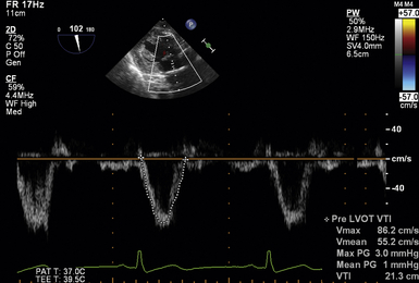
Figure 14-17 Obtaining left ventricular outflow tract (LVOT) velocity-time integral (VTI). Image obtained in deep transgastric long-axis view with pulsed wave cursor placed just proximal to aortic valve. Once obtained, velocity curve is traced, producing a peak and mean gradients and VTI within LVOT.
The VTI through the AV can be obtained using CWD to interrogate trans-AV flow in the deep TG LAX or TG LAX views (identical to obtaining a peak or mean gradient) and using the echocardiographic software package to trace the velocity curve. If a well-defined second lower velocity envelope is seen within the CW envelope used for the AV interrogation, this second velocity profile can then be used as the LVOT velocity envelope. The “double envelope” technique has the advantage of using a single cardiac ejection and minimizing the effects of beat-to-beat variability (see Fig. 14-15). The obtained velocity will represent the highest LVOT velocity, which owing to flow convergence should correspond to a site immediately proximal to the valve.
After obtaining all three measures, the cross-sectional area of the AV in cm2 can be solved for:
The continuity equation can also be simplified by substituting the VTI of the LVOT and AV with their respective peak velocities. Finally, the velocity or VTI ratio is a dimensionless measure comparing the peak velocity in the LVOT to that of the valve itself. A lower ratio signifies more severe stenosis. 22 The advantage of this technique is avoiding errors associated with incorrect LVOT diameter measurement:
Interpreting Results
Obtaining data regarding the severity of aortic stenosis is only part of the echocardiographic evaluation of aortic stenosis. Proper interpretation is a critical component of the examination as well. Because patients may present with widely varying body habitus, any calculated valve area should be indexed to patient size. This is particularly important for equivocal cases. Classification of valve stenosis based on indexed effective orifice area has been previously published ( Table 14-1). The ability to properly index valve area in patients with obesity remains a challenge.
TABLE 14-1
Quantification of Aortic Stenosis Severity
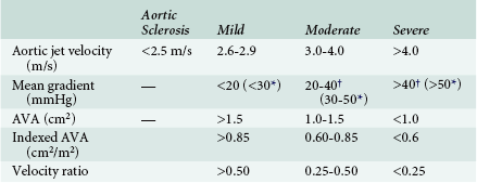
From Baumgartner H, Hung J, Bermejo J, et al. Echocardiographic assessment of valve stenosis: EAE/ASE recommendations for clinical practice. J Am Soc Echocardiogr. 2009;22:1-23.
Even with proper valve interrogation and area indexing, the clinical picture may remain equivocal in some cases. There are several reasons why this occurs. An important yet often overlooked factor is the effect of the “pressure recovery” phenomenon. The nature of fluid dynamics through a stenotic valve (discussed earlier) causes recovery of pressure distal to a stenosis to always occur. However, the degree of this recovery can vary considerably depending on several factors. Because Doppler techniques only measure the largest difference in velocity (and thus pressure) that occurs between the LVOT and vena contracta, any significant recovery of pressure distal to the valve is not appreciated. In contrast, because of the obligatory displacement of the catheter tip away from the vena contracta, the gradient measured by cardiac catheterization is a fundamentally different quantity than the Doppler-derived gradient. 23 The presence of elevated Doppler-derived gradients compared to catheter gradients—which cannot be explained simply by differences in peak-to-peak versus instantaneous measurements—have been demonstrated in some subsets of patients.24,25
where EOA is the effective orifice area and CSA is the cross-sectional area.
However, this formula has not been well validated. One of the biggest issues is that it does not account for several factors that affect the degree of pressure recovery. For example, the degree of jet flow angulation is believed to be an important variable. 17 In addition, in patients with no or mild stenosis, viscous forces likely predominate over the effects of pressure recovery, making the formula inapplicable in these patients. 26 Although the ability to accurately account for pressure recovery effects may be limited, it is important to consider its presence when making clinical decisions in patients with borderline surgical indications.
When evaluating the clinical significance of aortic stenosis, it is important to consider how the disease process affects the left ventricle and vice versa. The adaptation of the left ventricle to chronic pressure overload is increased ventricular mass due to chamber hypertrophy. The degree of hypertrophy and presence of diastolic dysfunction should be noted. Ventricular systolic dysfunction can develop later in the course of the disease. In patients with ventricular dysfunction and concomitant aortic stenosis, it is important to exclude the presence of pseudosevere aortic stenosis, which may occur secondarily to contractile dysfunction, leading to a reduced force of valve opening. With the semirigid leaflets seen in moderate (but not necessarily severe) stenosis, this reduced force may lead to valve area calculations consistent with severe stenosis even though the actual valve disease is not truly severe. This distinction may be significant, since pseudosevere aortic stenosis likely portends a worse prognosis. An inotropic challenge may help differentiate pseudosevere stenosis from severe stenosis, 27 but questions regarding individual variability in flow improvement exist. 28
It is also necessary to consider the interaction of the valve and the aorta. Poststenotic aortic dilation is not an uncommon finding ( Fig. 14-18). In addition, the association of bicuspid AV with ascending aortic aneurysm is well known. 29 The resulting “pressure drop” or energy loss across an AV stenosis may be exacerbated in patients with ascending aortic aneurysm. Consequently, these patients may develop symptomatic aortic stenosis despite relatively large AV orifice areas.
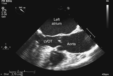
Figure 14-18 Poststenotic aortic dilation; transesophageal echocardiographic image obtained from midesophageal aortic valve long-axis view, showing patient with aortic stenosis and dilation (diameter 3.7 cm) of ascending aorta. LVOT, Left ventricular outflow tract.
Patients with senile degenerative aortic stenosis often have concomitant decreased arterial compliance, since both disease processes share histologic features consistent with atherosclerotic disease. 28 Patients who have reduced arterial compliance with aortic stenosis experience even greater left ventricular afterload elevations and will typically develop worsening compensatory hypertrophy. 30 The resultant smaller chamber size and afterload elevation may limit stroke volume, which might lead to lower peak and mean velocities than would be expected for a given degree of stenosis.
Stay updated, free articles. Join our Telegram channel

Full access? Get Clinical Tree


