Spatial Localization and Introduction to k-Space
If a subject were placed into the magnet bore and subjected to an RF pulse at the Larmor frequency, then all the protons in the bore would become excited. Without the use of gradients, the protons would generate one collective signal measurable by the receiver coils (Figure I5-1). This signal would include contributions from the entire body, without any differentiation based on location. Such a signal could not be used to make an MR image, because to make an MR image, spatial localization is required.
Spatial localization is the essential process of any imaging test. Signal must be differentiated based on location so that a spatial map of the signal can be presented as a diagnostic image. In MRI, this is achieved primarily with magnetic field gradients, which are applied in clever ways and at strategic times during the MR pulse sequence. For 2D imaging, spatial localization can be considered in three steps. First, slice-select gradients are used so that only a thin slice of tissue is excited and emits signal. Then, to localize signal within a given slice, two sets of gradients are applied: frequency-encoding gradients during the echo, and phase-encoding gradients at some time between the RF pulse and the echo. Standard descriptions of a 2D pulse sequence assume a transverse slice orientation. Slice-selective excitation is therefore performed using gradients in the z direction, frequency encoding with x gradients, and phase encoding with y gradients (Figure I5-2). But in real applications, these three orthogonal directions are freely interchangeable. For 3D imaging, excitation can be performed using slab-selective excitation or nonselective excitation. Then spatial localization is performed using one frequency-encoding gradient and two sets of phase-encoding gradients.
This chapter uses conventional explanations to describe spatial localization. Imaging artifacts that are associated with each step in spatial localization are also reviewed. In the next chapter, spatial localization will be revisited, with a view toward a deeper understanding of the wonders of k-space.
KEY CONCEPTS
[right half black circle] The goal of spatial localization is to identify the origins of signal on a voxel-by-voxel basis to generate a spatial map of signal intensity.
[right half black circle] Signal intensity values are determined for each voxel with coordinates x, y, and z, by using magnetic field gradients in the x, y, and z directions.
[right half black circle] Linear gradients cause Larmor frequencies to change linearly with distance along the direction of the gradient.
[right half black circle] For 2D imaging, localization in the z direction is achieved by slice-selective excitation. A slice-select gradient is applied during RF excitation; the thickness of the slice and its profile depend on the slice-select gradient strength, the transmitter bandwidth, and the nature of the RF excitation pulse.
[right half black circle] Localization in the x direction is accomplished using a frequency-encoding gradient, while localization in the y direction requires a phase-encoding gradient.
[right half black circle] The echo is sampled during the frequency-encoding gradient; for accurate signal measurement, the sampling frequency must be at least twice as high as the largest frequency measured (the Nyquist theorem).
[right half black circle] Phase-encoding gradients are applied at times other than RF excitation and signal sampling.
[right half black circle] The dephasing caused by gradients can be reversed with rephasing lobes.
[right half black circle] Although the Larmor frequency for MR imaging is relatively high (64 MHz), MR RF pulses and signals are low frequency (Hz or kHz), subject to modulation and demodulation.
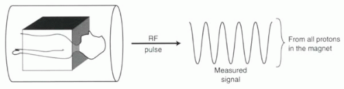 FIGURE I5-1. The challenge of spatial localization. Making MR images requires resolving which portions of the MR signal come from which parts of the body. |
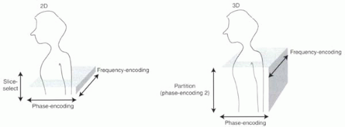 FIGURE I5-2. Standard nomenclature for 2D and 3D spatial localization, assuming an axial imaging 2D slice or axial 3D slab. |
Before beginning the discussion of spatial localization, it is necessary to review the concepts of modulation and demodulation. Although the Larmor frequency is about 64 MHz, most of the signals used to make MR images—the RF excitation pulses and the echoes or signals recorded—are actually much lower in frequency, on the order of kilohertz (kHz) rather than megahertz (MHz). (Recall that 1 kHz = 1000 Hz, while 1 MHz = 1,000,000 Hz.) Low-frequency RF pulses are modulated with the high Larmor frequency to achieve RF excitation, while the high-frequency echoes are demodulated back to lower frequencies for signal processing. The following Background Reading provides an introduction to the concepts of modulation and demodulation.
BACKGROUND READING: Modulation and Demodulation
The concept of modulation and demodulation is the key behind the function of a familiar household appliance, the AM/FM radio. AM stands for amplitude modulated signal, while FM is frequency modulated. Radios transmit sounds originating far away. The range of frequencies that comprise the human voice and music is approximately 1-2 kHz. How can these sounds be transmitted miles away? To transmit sound waves far distances, frequencies much higher than 1-2 kHz must be used. Think about the effect of standing atop a skyscraper (alongside a transmitter) and yelling at the top of your lungs. The total audience for your broadcast would be rather limited, and the competition with other broadcasters would be pretty fierce. On the other hand, higher frequencies, such as in the hundreds of kHz or tens of MHz range (AM 820 kHz or FM 93.9 MHz, for example) can travel miles and penetrate buildings, with minimal interference from other carrier frequencies. But the human ear cannot hear these frequencies.
Radios work because the lower frequencies of voice and music can be superimposed onto a high-frequency carrier wave. The radio transmitter achieves this by a process called modulation, which can be performed by amplitude modulation (Figure I5-3) or, as in the case of MRI, frequency modulation. The radio receiver removes the high carrier frequency and recovers the music by demodulation (Figure I5-3).
MR operates in a similar way. The RF pulse has a bandwidth of a few kHz, while the 64 MHz Larmor frequency is the carrier frequency. When transmitted, the RF pulse is modulated to a 64 MHz carrier frequency to achieve resonance. In terms of the echo produced, the high-frequency signal received is centered around 64 MHz, but for analysis the MR computer demodulates the signal into its low-frequency (kHz) components.
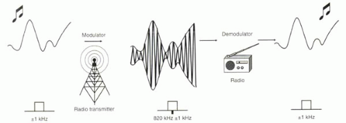 FIGURE I5-3. Radio transmission. Low-frequency music is modulated by a high carrier frequency required for transmission over long distances. The radio receives the signal and demodulates it back to the original low-frequency, audible, signal that is heard as music. The bandwidths of frequencies are depicted beneath each signal. (Note that in this example the signal is amplitude modulated. With MR, the signal is frequency modulated, which is harder to depict graphically, but conceptually rather similar.) |
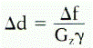
Z-AXIS LOCALIZATION: SLICE-SELECT GRADIENTS AND CROSS-TALK ARTIFACTS
For 2D imaging, RF excitation is performed during application of a slice-select gradient so that only tissue within a thin slice is excited and will subsequently generate signal. Slice-select gradients ensure that all of the measured signal will originate from the same position in the z direction (assuming a transverse slice). With slice-select gradients, the z coordinate for spatial localization is predetermined, and protons outside the desired coordinates do not contribute to signal intensity.
Slice-selective excitation takes advantage of the requirement for resonance. A linear magnetic field gradient in the z direction causes the magnetic field strength to vary along the z axis (Figure I5-4). If the RF pulse consists of a pure 64 MHz signal, then only a very thin slice of tissue at 1.5 T will be excited. All other protons will be oblivious to the RF excitation pulse because they do not fulfill resonance conditions.
CHALLENGE QUESTION: Why would this scenario of a perfect 64 MHz RF excitation pulse not be a desirable way to achieve slice-selective excitation?
View Answer
Answer: This scenario would not be desirable because the slice that would be excited by a pure 64 MHz pulse would be infinitesimally thin and contain too few protons to generate measurable signal for imaging.
A real RF pulse has a finite width and includes a range of frequencies. For example, the range might be from 63.998 to 64.002 MHz. The 0.004 MHz, or 4 kHz, range of frequencies is referred to as the transmitter bandwidth (Figure I5-4). (Note that this bandwidth is different from the more commonly encountered receiver bandwidth, which will be discussed later with frequency encoding.) Bandwidths in MRI are usually expressed as ±fmax kHz, where fmax is the maximum frequency in the range, so that a 4 kHz transmitter bandwidth could also be written as ±2 kHz.
Slice Thickness
The relationship between slice-select gradient strength, transmitter bandwidth, and slice thickness is explored in this section (Figure I5-5).
The gradient strength is the ratio of the change in magnetic field, ΔB0, over a given distance, Δd. For the slice-select gradient, Gz (mT/m),
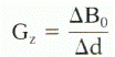
To relate ΔB0 to transmitter bandwidth, Δf, use the Larmor equation, f = γB, to yield Δf = γΔB. Substitute ΔB0 = Δf/γ,
Expressed in terms of slice thickness,
This equation says that to get thinner slices (smaller Δd), a lower transmitter bandwidth (Δf) and/or higher gradient strength (Gz) are necessary.
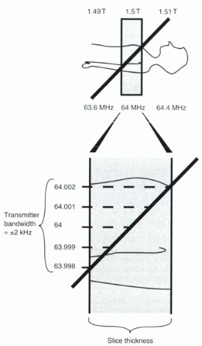 FIGURE I5-4. Slice-select gradient. A gradient is applied in the z direction so that protons are exposed to different magnetic fields along the length of the body and therefore precess at different frequencies. For a transmitter bandwidth of ±2 kHz, the slice that will resonate with the RF pulse will include all protons precessing at 63.998-64.002 MHz. A narrower transmitter bandwidth gives rise to a thinner slice. |
CHALLENGE QUESTION: Using a slice-select gradient of 20 mT/m to excite a slice with thickness 5 mm, what is the range of frequencies that should be included in the RF excitation pulse? What about a 10 mm slice?
RF Pulses, Fourier Transforms, and Slice Profiles
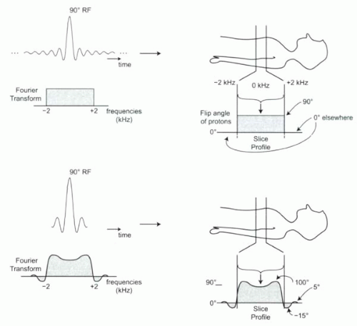
One important concept in slice-selective excitation is the slice profile. The slice profile describes the amount of excitation caused by a slice-selective RF excitation pulse, both within the desired imaging slice and beyond. An ideal slice profile for a 90° RF excitation pulse is depicted in Figure I5-6, where the tissues within the slice are tipped uniformly by 90°, while tissues outside the slice experience no excitation.
What is the relationship between the RF excitation pulse and the slice profile? It turns out that there is a one-to-one correspondence between the Fourier transform of the RF pulse and the slice profile (Figure I5-6, for example).
Recall from Chapter I-1 that the Fourier transform describes the relative amounts of signal at all the component frequencies of an RF pulse. During application of the slice-select gradient, these frequencies correspond to different locations along the slice-select direction. They define the boundaries of the slice to be imaged.
The amplitude component of the Fourier transform describes how much energy is contained in each frequency component of the RF signal. This in turn defines the extent of RF excitation achieved at each location within the slice.
If the contributions are uniform across the transmitter bandwidth, then the Fourier transform will be a perfect rectangle. The slice profile will also be “ideal.”
CHALLENGE QUESTION: What is the appearance and duration of the RF pulse that will result in perfect slice excitation?
IMPORTANT CONCEPT:
The Fourier transform of the RF pulse determines the excitation profile of the imaged slice. A rectangular Fourier transform corresponds to an “ideal” slice profile, where the slice is uniformly excited to the desired flip angle, without any excitation of tissue outside the slice. To achieve such a perfect excitation, the RF pulse would have to be an infinitely long sinc function.
Faster and Truncated Sinc RF Pulses and Their Slice Profiles
Long RF pulses are usually detrimental to MR imaging efficiency, and infinitely long RF pulses are clearly not practical. One useful feature of the sinc function is that most of the information in the curve is contained within the central peak and a few ripples to either side of the curve. Hence, the RF pulse can be truncated to reduce the time needed for RF excitation. RF pulse durations can be further reduced by the use of stronger slice-select gradients.
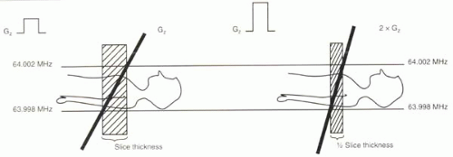 FIGURE I5-5. Slice thickness, transmitter bandwidth, and gradient strength. For a fixed transmitter bandwidth of ±2 kHz, the slice thickness can be halved by doubling the amplitude of the slice-select gradient. |
 FIGURE I5-6. “Ideal” RF pulse for perfect slice profile. The ideal RF pulse for exciting a slice is a sinc pulse. All protons within the slice are excited to 90°, whereas none of the tissue outside the slice is excited (0° flip angle). The transmitter bandwidth profile (left) represents a one-dimensional Fourier transformation of the RF pulse, as does the slice profile (right). |
To understand the effects of truncated RF pulses on slice profiles, more Background Reading is provided on sinc functions, truncated sinc functions, and their Fourier transforms. It is important to understand this section, because many of the themes will recur in the later section on receiver bandwidth and echo sampling.
BACKGROUND READING: Sinc Functions, Truncated Sinc Functions, and their Fourier Transforms
Sinc Functions
The sinc function is defined as f(x) = (sin x)/x (except at x = 0, where sinc x = 1). The sinc function plays a central role in MR imaging because MR signals and RF pulses commonly represent the sum of sinusoidal functions across a relatively narrow range of frequencies. The Fourier transform (FT) of any function is a histogram of the amounts of different frequencies that, when summed, generate the function (Chapter I-1). The range of frequencies used to generate a sinc curve is referred to as the bandwidth. Bandwidth is usually centered around the zero frequency (demodulated) and expressed as ±fmax kHz or 2fmax kHz, where fmax is the maximum frequency in the range. For example, a ±1 kHz bandwidth would mean that the range of frequencies includes −1 kHz through +1 kHz. This could also be expressed as a bandwidth of 2 kHz.
One useful property of sinc functions is worth reviewing. As shown in Figure I1-15 and Figure I5-7,
the wider the bandwidth comprised in the sinc function, the narrower the main peak of the sinc curve and the smaller the ripples. That is, at higher bandwidths the sinc function looks more and more “compressed.” The “compressed” appearance results from the contributions of the higher frequencies (Figure I1-15). This concept is extremely important and recurs throughout many topics in MR physics!
the wider the bandwidth comprised in the sinc function, the narrower the main peak of the sinc curve and the smaller the ripples. That is, at higher bandwidths the sinc function looks more and more “compressed.” The “compressed” appearance results from the contributions of the higher frequencies (Figure I1-15). This concept is extremely important and recurs throughout many topics in MR physics!
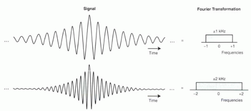 FIGURE I5-7. Two sinc functions with different bandwidths. Note that these functions are infinitely long. |
IMPORTANT CONCEPT:
Higher bandwidths correspond to more “compressed” sinc functions.
Truncated Sinc Function and its Fourier Transform
In an ideal world, to generate an RF pulse that contains an equal representation of all frequencies across the desired transmitter bandwidth, the RF pulse would have to be infinitely long in duration (note the “…” symbols on both sides of the sinc functions shown in Figure I5-7). But in MR imaging, time is always of paramount concern, so a long RF pulse is out of the question. In fact, “sinc” functions in MR are actually truncated sinc curves. Typically, the degree of truncation is defined in terms of the numbers of periods (full oscillations from positive to negative to positive peak) that are included in the curve (Figure I5-8).
What happens to the Fourier transform of the sinc function when it is truncated? It no longer has the appearance of a perfect rectangle. Rather than a uniform contribution of all frequencies within the bandwidth, the truncated sinc function becomes a variable mix of different amounts of different frequencies in the bandwidth and also starts to include some frequencies above and below the desired bandwidth (Figure I5-9).
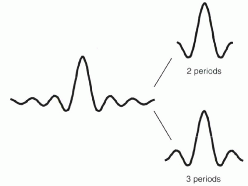 FIGURE I5-8. Truncated sinc function. Truncation of a sinc function is usually defined in terms of number of periods of oscillation, that is, the number of time the curve traverses one cycle of maximum-minimum-maximum. |
IMPORTANT CONCEPTS:
The Fourier transform of a sinc function of infinite duration is a rectangular function. Truncation of a sinc function leads to distortion of the rectangular Fourier transform—the more severe the truncation, the larger the distortion. Truncation and its effects are determined by the number of periods included in the sinc function.
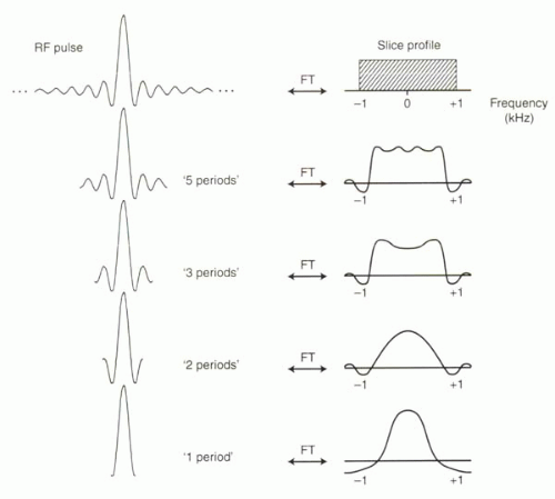 FIGURE I5-9. Fourier transforms of truncated sinc functions. The appearance of the Fourier transform depends only on the number of periods in the truncated sinc function within the pulse duration and not on the duration of the pulse. |
What happens to the slice profile when a sinc RF pulse is truncated? A truncated RF pulse will cause some parts of the slice, such as the center, to be excited as desired, but other areas, such as the edges, will be excited either more or less than expected. In addition, there may be excitation outside the slice (Figure I5-10). Imperfect excitation means that an RF pulse intended to cause a 90° flip angle may cause a 100° flip angle at the edges of the slice. Outside the slice, where there should be no excitation, the truncated sinc RF pulse will cause small excitations (for example, ±15° flip angle). Although these effects may seem unimportant, they can dramatically affect image contrast and image quality.
The slice profile depends on the number of periods included in the truncated RF pulse and not necessarily on the actual duration of the RF pulse. By using stronger slice-select gradients, the time needed to include, say, three periods in the RF pulse can be shortened.
CHALLENGE QUESTION: Why do stronger slice-select gradients shorten the RF pulse needed to achieve a given slice profile?
View Answer
Answer: If slice-select gradients are stronger, then the transmitter bandwidth increases correspondingly for a given slice thickness. An RF pulse with higher transmitter bandwidth will be more “compressed” than that with a lower transmitter bandwidth. Since the slice profile is dependent only on the number of periods contained in the RF pulse, a higher-bandwidth RF pulse requires less time for the same number of periods or the same slice profile.
Two scenarios are illustrated in Figure I5-11. A certain slice-select gradient is applied across the body so that the transmitter bandwidth is ±1 kHz and excites a 5 mm thick slice with a 1 msec, two-period RF pulse. If the gradient strength is doubled, then the transmitter bandwidth for the same 5 mm thick slice would double to ±2 kHz. At this bandwidth, the RF pulse would look much more “compressed”; in fact, with double the frequencies, it would be twice as “compressed.” Two periods would now require only half as long, or 0.5 msec. Alternatively, if the RF pulse duration was maintained at the same 1 msec duration, the RF pulse would include four periods instead of two, resulting in a much improved slice profile with the stronger slice-select gradient.
 |
Stronger gradients can be used to advantage in one or a combination of the following three ways:
1. To reduce the RF pulse time: With double the slice-select gradient strength, the RF pulse duration in the example can be halved without sacrificing the quality of the slice profile.
2. To improve the slice profile: With double the gradient strength, the same RF pulse time of 1 msec will include four periods instead of two periods, resulting in a more rectangular slice profile.
3. To reduce the slice thickness: With double the gradient strength, if the original RF pulse transmitter bandwidth is maintained, then the excited slice will be half as thick at 2.5 mm. The quality of the slice profile will be identical to that of the original 5 mm slice.
IMPORTANT CONCEPT:
Strong slice-select gradients can be used to (1) reduce the duration of the RF pulse, (2) improve the slice profile of the same slice thickness, and/or (3) reduce the slice thickness.
Cross-Talk
Cross-talk artifacts are the effects of imperfect slice profiles on the imaging of neighboring slices. For 2D imaging, to ensure that small lesions are not missed, imaging would ideally be performed using a series of contiguous thin slices. With MR imaging, this would require that each 2D slice be excited uniformly, one at a time, without any stray excitation outside the desired slice (Figure I5-12). In fact, imperfect slice profiles caused by routine truncation of the RF pulses result in imperfect excitation


Stay updated, free articles. Join our Telegram channel
Full access? Get Clinical Tree
