Echoes
Most MR images can be characterized as either spin echo or gradient echo images. This chapter focuses on how each type of image is produced and their properties and explores the parameters that can be manipulated to alter image contrast with each approach. The techniques for reducing acquisition times for each type of sequence will be discussed. Finally, specific applications of spin echo and gradient echo sequences in cardiovascular MR imaging are introduced. More detailed explorations are covered in Sections II and III of this book.
KEY CONCEPTS
[right half black circle] Two main types of echoes are used for generating MR images: spin echoes and gradient echoes.
[right half black circle] Gradient echoes are generated following a single RF pulse that can have a flip angle of less than 90° and a pair of dephasing and rephasing gradients.
[right half black circle] Gradient echo images have T2* weighting; unlike spin echoes, the effects of magnetic field inhomogeneities are not eliminated with gradient echoes.
[right half black circle] Partial flip angle gradient echo imaging leaves residual longitudinal magnetization for subsequent repeated RF excitations to be performed in quick succession.
[right half black circle] With gradient echo images, the sequence parameters that affect image contrast are the repetition time (TR), echo time (TE), and flip angle.
[right half black circle] T1-weighted spoiled gradient echo images are generated with relatively long TR, short TE, and large flip angles, while T2*-weighted images rely on short TR, long TE, and small flip angles.
[right half black circle] Multiecho gradient echo acquisitions improve efficiency of gradient echo imaging.
[right half black circle] Steady-state free-precession gradient echo imaging using balanced gradients provides image contrast that is T2/T1 weighted and requires short TR (<5 msec) and homogeneous B0 magnetic field.
[right half black circle] Spin echo images are generated following two RF pulses (typically a 90° and a 180° pulse) and a pair of dephasing and rephasing gradients.
[right half black circle] With spin echoes, the two sequence parameters that affect image contrast are the TR, which determines T1 contrast, and the TE, which determines T2 contrast.
[right half black circle] T1-weighted spin echo images are produced using short TR and short TE, while T2-weighted images rely on long TR and TE.
[right half black circle] Fast spin echo imaging improves the efficiency of spin echo imaging by a factor equal to the echo train length (ETL), but at the price of reduced image contrast.
[right half black circle] Half-Fourier single-shot fast spin echo sequences generate images as fast as one second per slice, but are limited by high specific absorption rate (SAR), decreased T2-weighted image contrast, and relatively low signal-to-noise ratio.
[right half black circle] Spin echo imaging reduces the effects of B0 field inhomogeneities that cause T2′ decay, allowing intrinsic T2 relaxation differences to be visualized.
GRADIENT ECHOES
Gradient Echoes: The Concept
A gradient recalled echo (GRE), or gradient echo, is produced by the application of a pair of gradient pulses that serve to dephase and then partially rephase magnetic moments. The process of rephasing generates an echo within the free induction decay (FID) time; this echo is sampled or measured with the receiver coil and used to fill k-space. This chapter explains how gradient pulses generate echoes and affect image contrast. The methods for spatial encoding of gradient echoes will be discussed in Chapters I-5 and I-6.
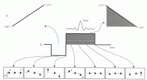 FIGURE I4-1. Gradient recalled echo. By first dephasing and then rephasing magnetic moments, the gradients produce a gradient echo. Protons that initially experience a magnetic field less than 1.5 T with the dephasing lobe (S, slow) will subsequently be exposed to a magnetic field greater than 1.5 T with the rephasing lobe (F, fast). In this example, maximum refocusing occurs at the midpoint of the rephasing lobe. |
The process of controlled, intentional dephasing and then rephasing of the magnetic moments is illustrated in Figure I4-1.
Controlled Dephasing
As introduced in Chapter I-2, following an RF excitation pulse, the transverse component of magnetization precesses about the xy plane with phase coherence. However, once the RF pulse ends, the magnetic moments begin to dephase, and the measured signal decays. With gradient echo imaging, a gradient that is applied during this process causes accelerated dephasing (Figure I4-1). By convention, the gradient is applied in the x direction.
Controlled Rephasing
To generate a gradient echo, a second gradient pulse is then applied, with reversed polarity. Wherever the dephasing gradient caused the field to be greater than 1.5 T, the reversed gradient causes it to be less than 1.5 T, and vice versa. Hence, protons that had been precessing more slowly will now precess faster, whereas those that had been faster will now be slower. Consequently, the rephasing gradient reverses the dephasing caused by the first gradient and brings the magnetic moments back in phase. At the moment of maximum phase coherence, the peak of the gradient echo is formed. If the reversed gradient is left on longer, accelerated dephasing will occur, and the echo will decay (Figure I4-2).
IMPORTANT CONCEPT:
Gradients always cause dephasing. Gradient echo imaging relies on controlled dephasing and then rephasing of magnetic moments.
The gradient echo is usually sampled during the entire duration of gradient reversal. The time between the peak of the RF pulse and the point of maximal refocusing (typically the midpoint of the gradient reversal) is called the echo time (TE) (Figure I4-2). The MR signals that are generated with gradient echo imaging are usually referred to as T2*-weighted because the amplitude of the echo is governed by T2* decay (FID) (Chapter I-2).
CHALLENGE QUESTION: If gradient echoes are affected by T2* decay, then is there truly perfect rephasing of the magnetic moments as illustrated in Figure I4-1?
View Answer
Answer: No! There will be some residual dephasing of the magnetic moments as a result of T2* decay, even at the peak of the gradient echo formation.
IMPORTANT CONCEPT:
Gradient recalled echo images have T2* weighting, which includes the effects of both field inhomogeneities and intrinsic T2 differences of tissues. Field inhomogeneity effects are not eliminated with use of gradient refocusing.
Gradient-Induced Phase Shifts
The amplitudes and durations of the dephasing and rephasing gradients are two parameters that can be varied in MR imaging. The question of how they affect the gradient echo process is explored in this section.
Gradients cause dephasing by inducing protons to precess at different frequencies along the direction of the gradient at different locations. The gradient amplitude determines how fast this dephasing occurs. The stronger the gradient, the faster the dephasing. For example, if a gradient with a particular amplitude G is applied for a duration t and causes the faster protons to be 90° ahead of the slower protons, then a gradient twice as strong, 2G, will accomplish the same phase difference in half the time. Alternatively, if the original gradient amplitude G is applied for twice as long, 2t, the protons will have twice the phase difference, or 180°.
This observation can be generalized by stating that the phase shift is proportional to both the strength of the gradient and the duration of the gradient. In mathematical terms, the phase shift, Δφ, for constant Gx, can be expressed as
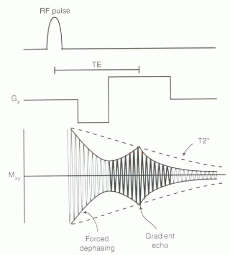 FIGURE I4-2. Formation of the gradient echo during T2* decay (free induction decay, or FID). The peak of the gradient echo occurs at a time called the echo time, TE, following the RF pulse. |
Δφ = 360° × Δft = 360° × γΔBgradientt = 360° × γxGxt
That is, Δφ depends on the difference in precessional frequencies, Δf, and the length of time, t, during which the frequencies are different. The frequency difference can be related to the magnetic field strength difference, ΔBgradient, by the Larmor equation, where γ is the gyromagnetic ratio. The field strength difference is in turn related to the gradient strength, Gx, and distance between protons, x, along the direction of the gradient.
When drawn in the format of a typical pulse sequence diagram, where the strength of the gradient is plotted as the height of the pulse and the duration is its length, phase shift can be considered as proportional to the area under the gradient curve (Figure I4-3).
Depending on the degree of dephasing desired, different combinations of gradient strengths and durations can be used, as illustrated in Figure I4-4.
Partial Flip Angle Imaging: A Free Lunch
With gradient echo imaging, a flip angle a of less than 90°, called a partial flip angle, can be used to shorten the time intervals between RF pulses (TR) and therefore to shorten the acquisition time.
How much transverse and longitudinal magnetization results from a partial flip angle RF pulse? Recall the relationship reviewed in Chapter I-1 (Background Reading on Vectors and Sines and Cosines) and illustrated in Figure I1-5. The magnitude of the transverse magnetization is equal to the magnitude of the magnetization vector, M, multiplied by the sine of the flip angle, sin α, while the longitudinal component is the magnitude multiplied by the cosine of the flip angle, cos α.
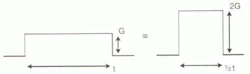 |
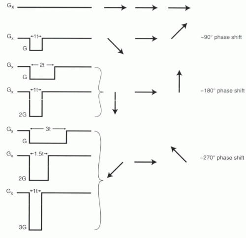 FIGURE I4-4. Relationship between gradient amplitude and duration and resulting degree of dephasing. |
IMPORTANT REVIEW POINT:
Any magnetization vector, M, can be expressed in terms of its transverse component in the xy plane, Mxy, which reflects measurable signal, and its longitudinal component, Mz, which represents stored or potential signal. The magnitude of each component is related to the flip angle, α, by the following equations:
Mxy = M sin α
Mz = M cos α
A Free Lunch
The “magic” of gradient echo imaging is that the sum of the magnitudes of the transverse and longitudinal magnetization components is greater than the magnitude of the original magnetization vector. Another way of thinking about this is to say that the sum of the lengths of the two sides of a right triangle are always greater than the length of the hypotenuse. (Note that this is a property of the magnitudes of the sides only; the sum of the two vectors, Mxy and Mz, exactly equals M.)
To get a better feeling for this relationship, consider a few examples of flip angles and the resulting longitudinal and transverse magnetization values in Figure I4-5 and Table I4-1.
Why is the partial flip angle such a useful feature? Following a partial flip angle excitation, a considerable amount of transverse magnetization can be generated for measurable signal. Yet, immediately following this excitation, there can still be substantial residual longitudinal magnetization for a subsequent excitation. For example, consider a 30° RF excitation pulse. For a net magnetization of amplitude M, the measurable signal in the transverse plane immediately after the excitation will have amplitude 0.5 M, while 0.87 M remains in the longitudinal direction. This means that a 30° RF pulse generates only half has much signal as would a 90° pulse, but it leaves 87% of the magnetization for another 30° RF pulse.
IMPORTANT CONCEPT:
Partial flip angle gradient echo imaging amounts to a “free lunch” because the sum of the magnitudes of the transverse and longitudinal magnetization components can exceed the magnitude of the original net magnetization. Following partial flip angle excitation, residual longitudinal magnetization (the amount depending on the flip angle, α) is available for a subsequent RF pulse.
Reaching Equilibrium with Gradient Echo Pulse Sequences
In many applications of gradient echo imaging, partial flip angle RF pulses are applied in quick succession without sufficient time for full T1 recovery between each pulse (Figure I4-6). The state of transverse and longitudinal
magnetization evolves over the first several RF excitations, after which a steady-state equilibrium is reached. The magnetization at equilibrium depends on the balance between two factors: the decrease in longitudinal magnetization resulting from each RF excitation and the amount of recovery of longitudinal magnetization during the time between successive RF excitations, called the repetition time or TR (Figure I4-6). Recovery depends on the relationship between the T1 relaxation time of tissues and the TR. With larger flip angles, more of the longitudinal magnetization is lost with each RF pulse. With longer TRs, shorter T1 relaxation times, or both, more is recovered in each interval.
magnetization evolves over the first several RF excitations, after which a steady-state equilibrium is reached. The magnetization at equilibrium depends on the balance between two factors: the decrease in longitudinal magnetization resulting from each RF excitation and the amount of recovery of longitudinal magnetization during the time between successive RF excitations, called the repetition time or TR (Figure I4-6). Recovery depends on the relationship between the T1 relaxation time of tissues and the TR. With larger flip angles, more of the longitudinal magnetization is lost with each RF pulse. With longer TRs, shorter T1 relaxation times, or both, more is recovered in each interval.
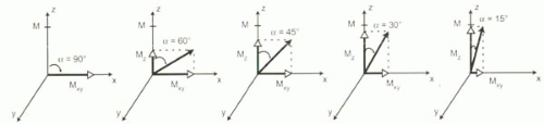 FIGURE I4-5. Longitudinal and transverse magnetization following RF pulses of 90°, 60°, 45°, 30°, and 15°. |
[right half black circle] TABLE I4-1 | ||||||||||||||||||||||||||||
|---|---|---|---|---|---|---|---|---|---|---|---|---|---|---|---|---|---|---|---|---|---|---|---|---|---|---|---|---|
| ||||||||||||||||||||||||||||
Figure I4-6 also shows how the flip angle affects the equilibrium that is reached. Immediately after each 30° pulse, Mz is 0.87 M, where M is the prepulse magnetization, while the magnitude of the transverse component, Mxy, is 0.5 M. In this example, some T1 recovery occurs during the TR interval, but it is not complete. Therefore, at the time of the second RF pulse, M, has not fully recovered to M. If it has recovered to 0.94 M, then following the next 30° RF pulse, the transverse component will be half of 0.94 M, or 0.47 M, while the longitudinal component will be 0.87 × 0.94 M, or 0.82 M. After several RF pulses, a balance is achieved at which the recovery of M, through T1 relaxation during the TR is equal to the amount by which it is decreased by each RF pulse.
In the same example, consider what happens if the flip angle is increased to 60°. Following each RF pulse, M, is 0.5 M, while the magnitude of the transverse component, Mxy, is 0.87 M. That is, the fraction of the longitudinal magnetization that is converted to measurable signal is considerably higher following a 60° pulse than following a 30° pulse. However, because the T1 relaxation of the tissue shown in this example is long relative to the TR, longitudinal recovery is modest in each repetition time. Therefore, the equilibrium is established at a much lower level of longitudinal magnetization. Consequently, the actual measured signal will be less with 60° RF pulses than with 30° pulses. The dampening of signal by repeated RF excitations in gradient echo imaging is commonly referred to as saturation. As shown in Figure I4-6, saturation is greater with higher flip angle excitations.
IMPORTANT CONCEPT:
After repeated partial flip angle excitations, a balance is achieved between the decrease in longitudinal magnetization resulting from each RF excitation and the longitudinal recovery that takes place during the interval between RF pulses.
Maximizing Signal in Gradient Echo Imaging
The maximum signal for a given tissue with known T1 value can be achieved when the following relationship between flip angle, αE, TR, and T1 is fulfilled:
cos αE = e−TR/T1
The optimal flip angle, αE, is known as the Ernst angle. When the TR is much larger than T1, then αE approaches 90°. On the other hand, when the TR is much smaller than T1, then the optimal flip angle αE is small and close to 0°.
Image Contrast: Balance between Flip Angle, TR, and T1
Figure I4-6 illustrates the effects of flip angle on one tissue. Parameters that are important for image contrast are TR, TE, and the T1 of tissues. To gain some insight into how TR, TE, and flip angle can be used to bring out differences due to tissue T1 and T2 relaxation times, consider the
following three commonly used versions of gradient echo sequences in cardiovascular MRI:
following three commonly used versions of gradient echo sequences in cardiovascular MRI:
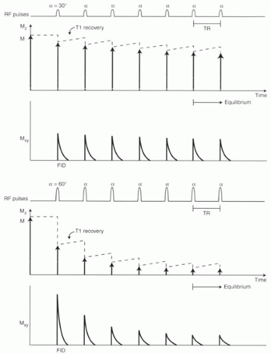 FIGURE I4-6. Longitudinal magnetization (Mz) and transverse magnetization (Mxy) after a series of RF pulses causing (a) 30° and (b) 60° flip angle. |
A. Long TR and Large Flip Angle
With gradient echo imaging, even a long TR is usually shorter than the T1 relaxation times of most tissues. Nevertheless, a long-TR sequence allows tissues with short T1 times to recover a substantial amount of longitudinal magnetization compared to tissues with long T1 times. If enough time is available for longitudinal recovery, then higher flip angles can be used without saturating the signal. Figure I4-7 illustrates the effect of long TR and large flip angle on tissues with short and long T1 values.
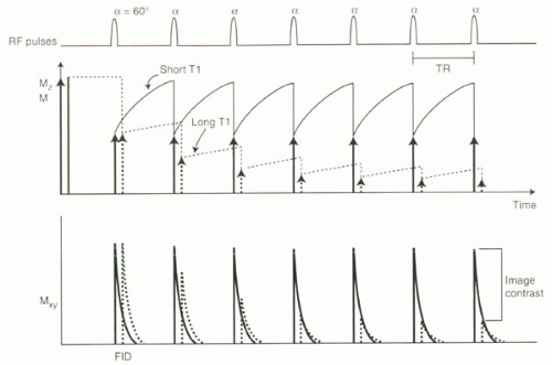 FIGURE I4-7. Gradient echo sequence with long TR and large flip angle results in image contrast for tissues with differing T1 relaxation times (short T1, solid line; long T1, dashed line). |
With long TR times, differences in T1 times are brought out because there is enough time for differences in longitudinal recovery to become apparent. The longer the TR times relative to the T1 recovery times, the higher the flip angle that can be used without saturating signal.
B. Short TR and Small Flip Angle
If TR is much shorter than T1, then there will be no significant recovery between each RF pulse. This means that the signal will simply depend on the flip angle, and there will be very little contrast based on differences in tissue T1 times. A high flip angle will lead to minimal residual longitudinal magnetization after each pulse and, consequently, very low signal (Figure I4-6). If TR is much less than T1, a small flip angle is usually used (Figure I4-8).
C. Gadolinium-Enhanced Imaging
Gadolinium-enhanced MR imaging provides a third option of generating contrast. The T1-shortening effects of gadolinium contrast material are dramatic. For gadolinium-enhanced MR angiography, the T1 of blood can become as short as 20 msec. As illustrated in Figure I4-9, because the recovery of longitudinal magnetization is so fast with gadolinium contrast material, short TR times and higher flip angles can be used.
CHALLENGE QUESTION: How can the contrast between gadolinium-enhanced tissues and background unenhanced tissues be further increased?
View Answer
Answer: By increasing the flip angle. Recall that gadolinium contrast material acts by shortening T1 relaxation times of the protons around it. If T1 is sufficiently short, then longitudinal magnetization of gadolinium-containing tissues will recover sufficiently even with high flip angles. However, with larger flip angles, the background tissues will become almost completely saturated and generate minimal signal. As a consequence, the contrast between gadolinium-enhanced tissues and background tissues will be even greater than the contrast at low flip angle.
IMPORTANT CONCEPT:
A long TR and a larger flip angle bring out differences in T1 relaxation times with gradient echo imaging. Conversely, shorter TR and a smaller flip angle minimize T1 weighting. Gadolinium-enhanced imaging favors a short TR and a larger flip angle to maximize contrast between gadolinium-enhanced vessels and other tissues.
Acquisition Times for Gradient Echo Imaging
How long does it take to make a gradient echo image? Following each RF excitation, a gradient echo is used to
fill a single line of k-space. For 2D imaging, to fill an entire 2D k-space, many echoes—typically 128 to 256—need to be collected. For reasons that will be more apparent in the next chapter, the number of echoes is referred to as the number of phase-encoding steps, NPE. The total time needed to acquire enough data to make an image, the acquisition time or Tacq, depends on NPE and on the repetition time TR. That is,
fill a single line of k-space. For 2D imaging, to fill an entire 2D k-space, many echoes—typically 128 to 256—need to be collected. For reasons that will be more apparent in the next chapter, the number of echoes is referred to as the number of phase-encoding steps, NPE. The total time needed to acquire enough data to make an image, the acquisition time or Tacq, depends on NPE and on the repetition time TR. That is,
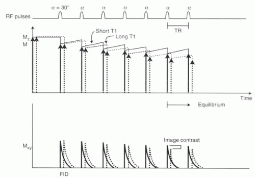 FIGURE I4-8. Gradient echo sequence with short TR and small flip angle minimizes differences in signal amplitudes for tissues with different T1 relaxation times (short T1, solid line; long T1, dashed line). |
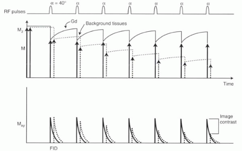 FIGURE I4-9. Gadolinium enhanced gradient echo imaging. The short T1 relaxation time of tissue containing gadolinium ensures that its signal is significantly higher than that of tissues with longer T1 times, despite high flip angles. |
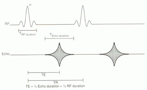 FIGURE I4-10. With fast gradient echo imaging, the TR is only slightly longer than the TE. Consequently, methods that reduce the TE will in turn reduce the TR and shorten acquisition times. |
for 2D gradient echo imaging. Therefore, short TR times are necessary for fast gradient echo imaging.
What are the factors that contribute to the TR for a gradient echo sequence? As illustrated in Figure I4-10, the TR is related to the duration of the RF pulse, the duration of the echo, and the TE.
Fast Imaging with Gradient Echoes
How short can the TR of a gradient echo sequence be? Because residual longitudinal magnetization after a partial flip angle RF pulse may be sufficient to allow a repeat excitation almost immediately after an echo is sampled, the TR does not need to be much longer than the TE (Figure I4-10). The TE for gradient echo imaging can be as short as 1 msec or less with MR systems that have strong gradients and fast slew rates. Corresponding TR times can be as little as 2 msec or even less.
Very short TRs mean fast imaging, because the acquisition time for an MR image is directly proportional to TR. With a short TR, acquisition times can be a fraction of a second for 2D imaging and less than 10 seconds for 3D imaging.
As will be more fully explored in Chapter I-8, these very short TR and TE times are achieved by minimizing the duration of each component of the pulse sequence that contributes to TR. In this section, the technique of shortening the TE by reducing the duration of the dephasing lobe of the gradient echo is illustrated.
IMPORTANT CONCEPT:
With gradient echo imaging, especially 3D gradient echo sequences, the TR need only be slightly longer than the TE. Therefore, methods that shorten TE will also shorten TR and hence reduce acquisition times.
Shortening the Dephasing Lobe
For gradient echo sequences, the echo is sampled only during application of the rephasing gradient. For reasons that will be discussed in subsequent chapters, the duration of this sampling period must be adequate to achieve desired signal-to-noise ratios and spatial resolution. Since no signal is measured during the dephasing lobe of the gradient, dephasing can be made as short as possible.
CHALLENGE QUESTION: How is it possible to have a shorter dephasing duration?
View Answer
Answer: Make the dephasing gradient amplitude stronger than that of the rephasing gradient (Figure I4-11).
The duration of the dephasing lobe is dependent on the maximum gradient strength of the system. The stronger the gradients, the shorter the dephasing duration. Why is this helpful? From Figure I4-2, the shorter the dephasing lobe, the shorter the echo time. As illustrated in Figure I4-11, shorter echo times can directly translate into faster repetitions of the gradient echo process, thereby leading to shorter acquisition times for MR imaging.
IMPORTANT CONCEPT:
For faster imaging, stronger gradients are advantageous because the same degree of dephasing can be achieved in shorter times, leading to shorter TE. With some gradient echo sequences, a shorter TE translates into shorter TR and consequently, shorter acquisition times.
Spoiled versus Steady-State Gradient Echo Imaging
With gradient echo imaging, the TR times can be shorter than the T2* of most tissues. This means that the transverse magnetization may not have fully decayed before
the next RF pulse occurs. Residual transverse magnetization can be troublesome because, after the next RF pulse, it is tipped away from the xy plane and contributes to longitudinal magnetization. Subsequent RF pulses may tip it into the transverse plane again. If this process is not well controlled, the contribution of the transverse magnetization to the measured signal can easily corrupt the image contrast and cause the so-called band artifact (Figure I4-12). The easiest way to solve this problem is to eliminate all the transverse magnetization before the subsequent RF pulse, a process called spoiling. These sequences are referred to as spoiled gradient echo sequences. So far, the discussion in this chapter has assumed spoiled gradient echo imaging. However, it is important to differentiate between spoiled gradient echo and another type of gradient echo imaging commonly used in cardiovascular MR imaging, known as steady-state gradient echo imaging. (Manufacturers have different terminology for each, as summarized in Table I4-2.) The distinction between the two types of gradient echo sequences is based on what happens to the transverse signal that has not fully decayed before the next RF pulse.
the next RF pulse occurs. Residual transverse magnetization can be troublesome because, after the next RF pulse, it is tipped away from the xy plane and contributes to longitudinal magnetization. Subsequent RF pulses may tip it into the transverse plane again. If this process is not well controlled, the contribution of the transverse magnetization to the measured signal can easily corrupt the image contrast and cause the so-called band artifact (Figure I4-12). The easiest way to solve this problem is to eliminate all the transverse magnetization before the subsequent RF pulse, a process called spoiling. These sequences are referred to as spoiled gradient echo sequences. So far, the discussion in this chapter has assumed spoiled gradient echo imaging. However, it is important to differentiate between spoiled gradient echo and another type of gradient echo imaging commonly used in cardiovascular MR imaging, known as steady-state gradient echo imaging. (Manufacturers have different terminology for each, as summarized in Table I4-2.) The distinction between the two types of gradient echo sequences is based on what happens to the transverse signal that has not fully decayed before the next RF pulse.
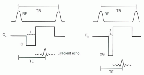 FIGURE I4-11. Stronger dephasing gradients lead to shorter TE and TR. The dephasing lobe is shortened by using the strongest possible gradients. |
The concept behind steady-state gradient echo imaging is that under certain circumstances, the residual transverse magnetization can actually be used to increase the measured signal. Recent advances in technology have enabled the application of steady-state gradient echo imaging to body and cardiovascular MRI, with major improvements in image signal-to-noise and contrast-to-noise ratios in shorter imaging times.
More specifics about each type of gradient echo sequence are provided in the following two sections.
Spoiled Gradient Echo Imaging
The three most commonly used ways to spoil a gradient echo sequence are as follows:
1. Long TR: If TR is more than 3 to 4 times the T2 relaxation times—preferably greater than 500 msec, or at least greater than 200 msec—then the transverse magnetization will be spoiled by dephasing.
 FIGURE I4-12. Band artifacts (arrows) in gradient echo imaging resulting from undesired contributions of transverse magnetization to measured signal. |
2. RF spoiling: If a phase offset is added to each successive RF pulse (see Chapter I-2, Figure I2-9), then the
phases of the residual transverse magnetization vectors will cancel each other out because of their reduced coherence or wide distribution of orientations.
phases of the residual transverse magnetization vectors will cancel each other out because of their reduced coherence or wide distribution of orientations.
[right half black circle] TABLE I4-2 | ||||||||||
|---|---|---|---|---|---|---|---|---|---|---|
| ||||||||||
3. Spoiler gradients: The third approach to spoiling is to extend the duration of the readout gradient beyond the sampling of the echo and before the next RF pulse. The prolonged application of the gradient causes accelerated dephasing of the residual transverse magnetization (Figure I4-13). These extra gradient pulse durations are referred to as spoiler gradients or crusher gradients.
Out of these three, the spoiler gradient method is most commonly used.
Image Contrast in Spoiled Gradient Echo Imaging
In spoiled gradient echo imaging, the three main parameters that affect image contrast are the TR, the TE, and the flip angle. How these are used to achieve desired image contrast is described next.
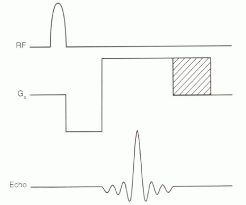 FIGURE I4-13. Spoiler or crusher gradient in a spoiled gradient echo sequence extends the rephasing lobe (dashed area) to “crush” residual transverse magnetization before subsequent RF excitation. |
Spoiled gradient echo images are usually either T1 or T2* weighted. With spoiled gradient echo imaging, true T2-weighted imaging is difficult to achieve because gradients, unlike 180° refocusing pulses in spin echo imaging (discussed later in this chapter), do not eliminate the loss of transverse magnetization caused by field inhomogeneities (T2*). The image contrasts that can be achieved by manipulating TR, TE, and flip angle are given in Table I4-3.
The longer the TR and the higher the flip angle, the more T1-weighted the image becomes. The longer the TE, the more T2*-weighted the image is (Figure I4-14).
IMPORTANT CONCEPT:
For spoiled gradient echo imaging, longer TR results in more T1 weighting, while longer TE causes more T2* weighting.
[right half black circle] TABLE I4-3 Spoiled Gradient Echo Imaging Parameters | ||||||||||||||||
|---|---|---|---|---|---|---|---|---|---|---|---|---|---|---|---|---|
|
 FIGURE I4-14. T2* weighting with gradient echo imaging. Metallic sternal wires accelerate T2* decay and cause the low signal of the wires to be exaggerated on this image. With the blooming artifact, the extent of signal loss (arrows) exceeds the region of the metal wires because the sequence used a long TE (9 msec). See also Figure I4-18. |
Signal intensity, SI, detected using gradient echo sequences can be expressed as the product of three factors that reflect the contribution of proton density, longitudinal recovery, and transverse decay. Recall from Chapter I-2 that the exponential recovery


Stay updated, free articles. Join our Telegram channel
Full access? Get Clinical Tree
