Phase Contrast MRI: Flow Quantification and MRA
Phase contrast imaging is primarily used to image blood flow, and therefore provides information that is more functional than anatomic. MR phase contrast data can be used for flow quantification by generating velocity maps, akin to Doppler ultrasound or echocardiography. They can also be used to make angiographic images as in phase contrast MR angiography. The first part of this chapter introduces the basic physics of phase contrast MR imaging. Applications to angiographic imaging and flow quantification are then discussed. Cardiac applications of phase contrast flow quantification are discussed separately in Chapter III-6.
KEY CONCEPTS
[right half black circle] With a bipolar gradient, protons moving in the direction of the gradient accumulate phase shift relative to stationary protons.
[right half black circle] Encoding velocity, or Venc, defines the range of velocities that can be measured with phase contrast flow quantification.
[right half black circle] Aliasing occurs if the tissue velocities exceed the Venc.
[right half black circle] Phase contrast angiography is sensitive to slow flow and features excellent background suppression.
[right half black circle] Phase contrast flow quantification sequences produce velocity-encoded images where signal intensity is proportional to the velocity of blood moving through or within the slice plane.
[right half black circle] The modified Bernouilli equation is used for estimating pressure gradients across stenoses based on the peak systolic velocity measured.
[right half black circle] Clinical Protocol:
[right half black circle] Aortic coarctation
PHASE CONTRAST MRI: THE PRINCIPLES
Recall from Chapter I-4 that for stationary protons, the dephasing caused by application of a gradient can be reversed by a gradient with opposite polarity. Such a pair of gradients with opposite polarity is referred to as a bipolar gradient.
Bipolar gradients have a different effect on protons depending on their motion along the direction of the gradient. This difference serves as the basis for phase contrast MR imaging and is used to generate image contrast between moving protons (such as blood in the vessels or heart) and stationary protons (most of the soft tissues).
The easiest way to understand phase contrast MRI is to consider the original implementation of the method using bipolar gradients, although, as will be discussed, other types of gradients are more commonly used now to make phase contrast images. The effects of bipolar gradients on stationary and moving protons are considered in turn.
Bipolar Gradients: Stationary Protons
A bipolar gradient is defined as a pair of gradient lobes with opposite polarity. For the discussion here, the amplitude of each lobe is equal but opposite in sign so that the areas under each lobe are assumed to be equal. As reviewed in Figure II3-1, a bipolar gradient causes no net phase shift for stationary protons (neglecting T2* decay).
Bipolar Gradients: Moving Protons
Now consider the effects of the bipolar gradient on protons moving in the direction of the gradient (Figure II3-2).
If a proton moves while the bipolar gradient is applied, then the amount of dephasing experienced will not equal the amount of rephasing. For example, consider a proton that moves from the neck to the pelvis during the course of the bipolar gradient application (Figure II3-2, top). During the positive lobe of the bipolar gradient, the proton in the neck will experience a stronger magnetic field, which causes a relatively large positive phase shift relative to the center of the magnet. It moves during this gradient, and by the time the gradient is reversed, it is in the lower abdomen and pelvis, where again it experiences a magnetic field that is greater than 1.5 T. Hence, during the reversed gradient, the proton continues to accumulate positive phase. At the end of the bipolar pulse, the moving proton will have a very large positive phase shift relative to the stationary protons in the field. The phase gain is directly proportional to the velocity along the direction of the gradient.
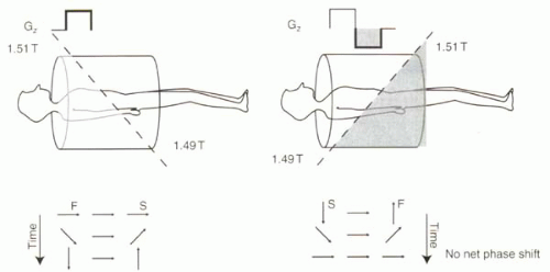 FIGURE II3-1. Bipolar gradient causes no net phase shift for stationary protons. Application of positive and negative gradients causes protons to precess relatively fast (F) and slow (S) depending on their position along the gradient. When the areas under the positive and negative gradient lobes are equal, stationary protons exhibit no net phase shift. |
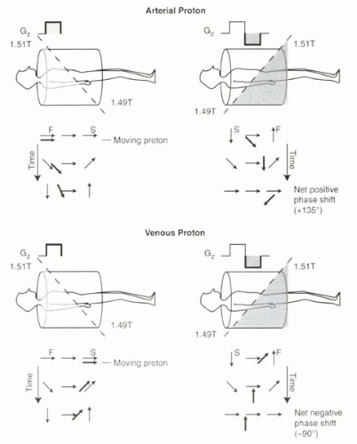 FIGURE II3-2. Bipolar gradient causes a net phase shift for moving protons. The arterial proton accumulates a positive phase shift during both lobes of the gradient and ends up with a net positive phase shift of 135°. The venous proton accumulates less phase shift than a faster-moving proton, and the phase shift is opposite in sign. |
What happens if the proton moves half as fast and travels from the neck to the abdomen during the course of the bipolar gradient? Again, during the positive lobe of the gradient, the proton will accumulate a positive phase shift. But during the reversed gradient, the proton will experience little rephasing in the center of the magnet. This means that at the end of the bipolar pulse, this slower proton will still have a positive phase shift relative to the stationary protons, but it will not be as great as the faster-moving proton.
What if the proton moves in the opposite direction, for example a proton in the veins (Figure II3-2, bottom)? The relative phase of the proton will now be negative compared to the center of the magnet. During the reversed gradient, the rephasing will be minimal, and hence the venous proton will then have accumulated a negative phase shift.
These observations can be summarized as follows:
Stationary protons accumulate no net phase shift following application of bipolar gradients, provided each lobe has equal and opposite area.
The phase shift that is accumulated by moving protons is directly proportional to the speed of the protons moving in the direction of the bipolar gradient.
The phase shift is also dependent on flow direction. As illustrated in Figure II3-2, arterial and venous protons accumulate phase shifts with opposite sign.
The exact relationship between phase shift and velocity of the protons can be predicted for a given bipolar gradient. In this way, phase contrast MR imaging can be used to convert maps of phase shifts into velocity maps.
Phase shifts accumulate for moving protons only if the protons are moving in the direction of the gradients. The direction of the bipolar gradients is referred to as the flow sensitivity direction or the velocity-encoding direction. Protons moving perpendicular to the gradients will not experience any phase accumulation.
IMPORTANT CONCEPTS:
Bipolar gradients cause protons moving in the direction of the gradients to accumulate a phase shift that is proportional to the velocity. Protons moving in opposite directions have phase shifts of opposite sign.
Two Bipolar Gradients Needed for Phase Corrections in Phase Contrast MRI
For a single bipolar gradient to provide accurate measurements of velocity based on phase differences, all phase shifts must be solely attributable to movement of protons during the gradients. The magnetic field must be perfectly homogeneous and the gradients perfectly linear.
CHALLENGE QUESTION: What factors other than motion can cause phase shifts?
View Answer
Answer: Any factor that leads to differences in precessional frequencies across protons will produce phase shift. The most important contributor is magnetic field inhomogeneity.
Significant phase shifts are caused by magnetic field inhomogeneities, and these shifts are indistinguishable from those caused by motion. Consider the following example. If the main magnetic field is 1.5 T and the magnetic field gradient is intended to make the field at a particular location 1.51 T during the positive lobe and 1.49 T during the negative lobe, then a stationary proton would have no net phase shift after these two lobes of the bipolar gradient are applied. But what if the field is inhomogeneous, so that the magnetic field at a given location is 1.6 T instead of 1.5 T? Now the same bipolar gradient will cause the field at that location to be 1.61 T and 1.59 T during the two lobes. Relative to the protons that are at 1.5 T in the center of the magnet, the stationary protons in this region will experience a positive phase shift—a very positive phase shift—after the bipolar gradient. Thus, as a consequence of magnetic field inhomogeneity, these stationary protons would be misinterpreted as very fast-moving protons!
Therefore, without perfect field homogeneity it is impossible to do accurate phase contrast flow quantification using a single bipolar gradient. To correct for other causes of phase shifts, the collection of phase data with one bipolar gradient is repeated with following application of the mirror image of that bipolar gradient, and the two datasets subtracted (Figure II3-3).
The effect of field inhomogeneity on the net phase shift from each bipolar gradient will not be zero, but it will be the same for each bipolar gradient. In the example just described, the bipolar gradient that causes 1.61 T and 1.59 T would lead to a positive phase shift of, say, +160°. Then the second bipolar gradient, a mirror image of the first, would cause the field to be 1.59 T and 1.61 T, again resulting in a phase shift of +160°. Consequently, if the phase shifts from the two bipolar gradients are subtracted, then the net phase shift will be zero and the effects of an inhomogeneous magnetic field eliminated.
IMPORTANT CONCEPT:
To correct for magnetic field inhomogeneities, two separate sets of phase data using two different bipolar gradients are acquired and subtracted for phase contrast imaging.
For phase contrast flow quantification, two complete sets of echoes must be collected, one using each bipolar gradient. Having to repeat the acquisition and collect two sets of echoes makes phase contrast acquisitions twice as long as conventional gradient echo imaging.
CHALLENGE QUESTION: How many sets of acquisitions are necessary to generate a phase contrast image with flow sensitivity in three directions if bipolar gradients are used?
View Answer
Answer: With standard bipolar gradients, a pair of bipolar gradients are necessary in each encoding direction. This means that six separate acquisitions are needed for flow sensitivity in three directions.
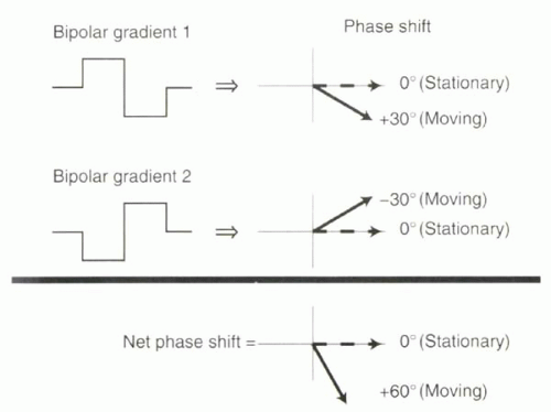 FIGURE II3-3. To correct for phase shifts arising from factors other than motion, two velocity-encoding gradients are applied and the two signals are subtracted. The phase shifts of moving protons will have opposite sign with the two sets of gradients, causing the net phase shift to double. |
Use of Flow-Compensated and Flow-Encoded Gradients
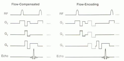
Subtracting two datasets is necessary to cancel out the phase errors due to field inhomogeneities. But the pairs of gradients need not be mirror-image bipolar gradients. In fact, on most commercial systems, phase contrast MR images are generated with phase images acquired with (a) flow-encoding gradients and (b) flow-compensated gradients (Figure II3-4). As with bipolar gradients, using this pair of acquisitions and subtracting one set of phase data from the other helps to reduce artifacts due to other causes of phase errors, such as field inhomogeneity.
Use of flow-compensated gradients reduces the number of acquisitions necessary to generate flow sensitivity in three directions to four. With conventional bipolar gradients, six acquisitions (one pair per direction) would be needed.
Flow Sensitivity Direction versus Imaging Plane
With phase contrast imaging, there is an important distinction between the direction of flow sensitivity and the plane of imaging.
For phase contrast MR angiography, there is often a need for flow sensitivity to be three-dimensional. Consequently, flow-compensated gradients are acquired in all three directions, and the entire sequence requires collection of four sets of data. The imaging plane or slab can be two- or three-dimensional.
Flow quantification acquisitions are typically 2D and set up to measure either in-plane flow or through-plane flow. Through-plane flow images are obtained by applying the velocity-encoding gradients in the slice-select direction (Figure II3-2), so that flow-sensitivity is in the through-plane direction, while the imaging plane is perpendicular to the direction of flow. Alternatively, the flow sensitivity desired may be in the plane of the image. In such cases, flow-encoding gradients are applied in both the frequencyand phase-encoding directions.
Three-dimensional phase–contrast flow quantification, with flow sensitivity in all three directions, is rarely used to image cardiovascular subjects because of the long acquisition times and complex image post-processing.
IMPORTANT CONCEPTS:
The direction of flow sensitivity and orientation of the imaging plane are independent parameters. With 2D flow quantification sequences, the direction of flow sensitivity can be either perpendicular to the imaging plane (“through-plane” with flow


Stay updated, free articles. Join our Telegram channel
Full access? Get Clinical Tree
