Overview of MRI and Basic Principles
The target audience for this book consists of radiologists, technologists, and others interested in medical imaging who want to understand how magnetic resonance (MR) images are made. The goals are to provide enough of a background in MR physics for the reader to use and optimize protocols for MR imaging (MRI), particularly cardiovascular MRI. Keeping in mind the rapid rate of innovation in the field of MRI, this book also aims to equip the reader with a sufficient foundation in MR physics to understand and incorporate future technological advances.
Section I of this book (Chapters I-1, I-2, I-3, I-4, I-5, I-6, I-7, I-8, I-9 and I-10) describes the general principles of MR physics. Section II puts these principles to practice in vascular imaging applications. Section III is devoted to cardiac imaging.
Section I is meant to be comprehensible to readers of all backgrounds. Although many theoretical principles are reviewed, the emphasis is always on their practical implications. Key mathematical and engineering ideas necessary to understand MRI are reviewed in Background Reading sections. Throughout the text, Challenge Questions are intended to engage the reader in the learning process. Take-home messages for each section are summarized in “Important Concepts.” New terms are italicized and defined in the Glossary at the end of this book. The main ideas of each chapter are summarized in “Key Concepts.”
This first chapter introduces foundational principles of MRI. The topics of this chapter are: the behavior of hydrogen protons as tiny oscillating magnets in an external magnetic field, the hardware components of an MR system, an overview of image formation, the characteristics of an image that define its quality, and an introduction to pulse sequence diagrams—the recipes for making MR images.
KEY CONCEPTS
[right half black circle] Human bodies are made of 95% water. Each water molecule consists of two hydrogen atoms and one oxygen atom.
[right half black circle] Hydrogen protons have a special property—they behave like tiny magnets.
[right half black circle] Magnetic properties of a single proton (its magnetic moment) or of an aggregate of protons (net magnetization) can be depicted as a vector that may change size and orientation over time.
[right half black circle] When placed in a steady magnetic field, the magnetization of protons will align with the field, and their magnetic moments will precess around the axis of the field at the Larmor frequency.
[right half black circle] Precessing protons can be depicted as spinning vectors whose frequencies can be expressed in units of hertz (Hz, cycles per second, denoted by f) or of radians per second (as denoted by ω), where ω = 2πf.
[right half black circle] Hydrogen protons in water molecules precess at different frequencies from those in fat molecules because of their different molecular environments.
[right half black circle] Radiofrequency excitation temporarily deflects magnetization from the direction of the external magnetic field. Afterward, magnetization will return to its initial direction via a process called relaxation.
[right half black circle] Radiofrequency excitation leads to the generation of MR signals, which are used to produce images; tissues have different appearances on MR images based, in part, on differences in their relaxation properties.
[right half black circle] To generate MR images, the positions of protons in the body are localized to specific parts of an image by means of magnetic field gradients and data processing using Fourier transformations.
[right half black circle] Defining characteristics of an image include its spatial resolution, signal-to-noise ratio, and contrast-to-noise ratio.
[right half black circle] Basic components of an MRI system include a superconducting magnet, transmitter and receiver coils, and gradient coils.
[right half black circle] A pulse sequence diagram is a recipe for generating an MR image. It describes the temporal coordination of radiofrequency excitation pulses, gradients, and signal measurements.
HUMANS AS PROTONS AND PROTONS AS MAGNETS
Each hydrogen nucleus consists of a single proton that can be considered as a simple magnet with a tiny magnetic field (Figure I1-1), referred to as its magnetic moment.
IMPORTANT CONCEPT:
Protons that constitute hydrogen nuclei behave like tiny magnets.
Although the magnetic field of a single proton is minuscule, the aggregate effect of hydrogen protons in the body is measurable. This is because approximately 95% of the body’s mass is water (H20). Every mole (18 grams) of water contains 6.023 × 10²³ oxygen atoms and twice as many hydrogen atoms. Thus, the body of an average 60 kg woman contains about 3.8 × 1027 hydrogen protons in water molecules, not including the protons in her fat!
While the nuclei of elements other than hydrogen, such as phosphorus, sodium, and fluorine, can also be used to generate MR images, the natural abundance of hydrogen in the body makes it particularly suitable for clinical imaging applications.
The generation of clinical MR images can be understood in terms of manipulations of the magnetization of hydrogen protons. Important concepts that will be discussed include the effects of large external fields on the magnetic moments of protons, the consequences of temporarily deflecting magnetic moments away from the direction of the large external field, and the magnetic moments’ return to an equilibrium state following the deflection. Each of these concepts requires an understanding of some of the principles of electromagnetism and electromagnetic induction, which are reviewed in the following Background Reading.
BACKGROUND READING: Electromagnetism and Electromagnetic Induction
A magnetic field can be generated in different ways. The most familiar form of a magnet is a bar magnet. It is usually made of iron, and one end of the magnet acts as the north pole while the other is the south pole. Alternatively, a magnetic field can be generated by passing an electrical current through a wire. Current flowing through a loop of wire generates a magnetic field perpendicular to its plane. If the wire is configured as a solenoid—that is, it is coiled tightly in a cylinder (Figure I1-2)—then the magnetic field induced along each loop of the solenoid is added to the fields induced along the other loops, and consequently a substantial magnetic field can be generated along the length of the cylinder. If the current passing through the solenoid is steady, then the magnetic field will be steady, with a north pole at one end of the coil and a south pole at the other end. The strength of the magnetic field is directly proportional to the amount of current passing through the wire and is referred to at B0 (“B zero” or “B naught”), typically measured in units of tesla or gauss, where 1 tesla (T) = 10,000 gauss (G).
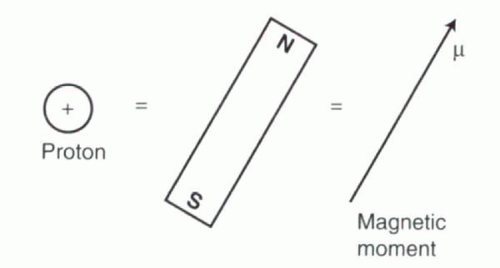 FIGURE I1-1. Protons as magnets. The proton that constitutes the nucleus of a hydrogen atom behaves like a tiny bar magnet. The magnetic field associated with the magnet, its magnetic moment, is expressed as a vector, μ. |
Electromagnetic Induction
Another important concept in electromagnetism is electromagnetic induction, which describes the effect of a magnetic field on a nearby wire. A magnetic field changing over time will induce current to flow through the wire (Figure I1-3). The pattern of current flowing through the wire will reflect the pattern of fluctuation of the magnetic field. For example, if the field changes at a particular frequency f, then the current induced in the wire will also alternate with frequency f. A steady magnetic field does not induce any current in the nearby wire.
IMPORTANT CONCEPTS:
Current flowing through a loop of wire or through a solenoid will generate a magnetic field. A changing magnetic field will induce current in a nearby wire.
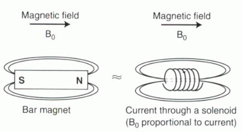 FIGURE I1-2. Electromagnetism. A magnetic field, B0, can be created using a bar magnet or by applying current through a coil of wire (solenoid). Note that the lines of flux representing the magnetic field of the solenoid are oriented along the bore of the coil (dashed lines). The magnetic field also extends around the solenoid, creating what is referred to as the fringe field. |
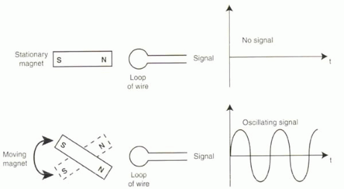 FIGURE I1-3. Electromagnetic induction. A static magnetic field (top) will not induce any current in a nearby loop of wire. However, a magnetic field changing over time (bottom) will induce a current in the loop of wire. The current will have the same frequency of oscillation as the magnetic field. |
MAGNETIZATION AS VECTORS
The magnetic properties of a single proton or a population of protons can be depicted as a vector, with a certain magnitude and direction. The magnetic moment of a single proton is often denoted as μ (mu) (Figure I1-1), whereas the cumulative effect of a population of protons is given by the net magnetization, M. The lengths of the vectors μ and M are referred to as their magnitudes, and their directions are usually defined as their angles with respect to some fixed set of reference axes. Before the behavior of magnetic moments in an external magnetic field is described, a review of vectors and sines and cosines is provided in the next Background Reading section.
BACKGROUND READING: Vectors and Sines and Cosines
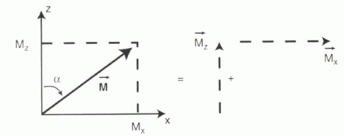
A vector is depicted as an arrow with a magnitude (or length) and angle (or orientation) with respect to some set of reference axes. Vectors can be constrained to lie within a plane (in which case they are called 2D) or they can point in any direction in space (in which case they are then called 3D). Any vector can be expressed as the sum of its x and y (for 2D) or x, y, and z components (for 3D). For example, a vector M in the xz plane with a magnitude M and angle α (alpha) relative to the z axis can be thought of as the sum of the x component, Mx, and the z component, Mz (Figure I1-4).
Similarly, a 3D vector M can be expressed as the sum of its x, y, and z components: M = Mx + My + Mz. In MR physics, the sum of Mx + My can be denoted as Mxy. Thus, M can be expressed as the sum of its z and xy components, M = Mz + Mxy (Figure I1-5). The angle that M makes with the z axis is usually referred to as α, while a second angle, φ (phi), describes the angle between Mxy and the x axis.
 |
To determine the relationship between the magnitude M, lengths of the components Mx and Mz or Mxy and Mz, and the angles α and φ, a review of sine and cosine functions is needed.
Definition of Sines and Cosines
A right triangle is defined as a triangle that has one 90° angle. Opposite the 90° angle is called the hypotenuse. Right triangles have useful properties that define the lengths of its sides relative to the angles formed by the sides and the length of the hypotenuse.
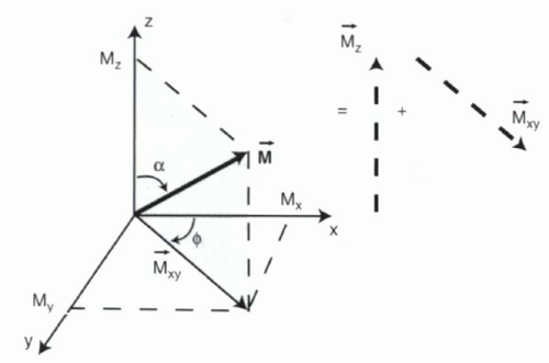 FIGURE I1-5. 3D magnetization vector. A 3D vector M can be represented as the sum of two components, Mz and Mxy, where Mz is considered the longitudinal magnetization, while Mxy is the transverse magnetization. |
For a right triangle (Figure I1-6), the sine (abbreviated as sin) of one of the non-90° angles is defined as the ratio of the length of the side opposite the angle divided by the length of the hypotenuse. The cosine (abbreviated as cos) of an angle is the ratio of the length of the adjacent side divided by the length of the hypotenuse. In other words, for the triangle in Figure I1-6,
sin α = Mx/M
cos α = Mz/M
These relationships are the same for all right triangles, regardless of size. Sine and cosine values for the entire range of angles have known values. These values can be used to determine the lengths of the sides of a triangle relative to the hypotenuse. Three sample α values are illustrated in Figure I1-6.
CHALLENGE QUESTION: What is sin 0? What is cos 0?
View Answer
Answer: As the angle α approaches zero, then Mx approaches zero, so sin 0 = 0. Mz approaches M, so cos 0 = 1.
From these definitions, it follows that for the 2D vector shown in Figure I1-4, the x and z components have magnitudes or lengths that can be predicted knowing the length of M and the angle a:
Mx = M sin α
Mz = M cos α
CHALLENGE QUESTION: For the 3D vector shown in Figure I1-5, what are the magnitudes of the two components Mxy and Mz in terms of the magnitude M and the angle α?
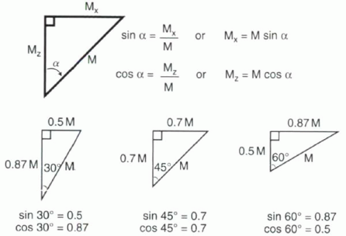 FIGURE I1-6. Sine and cosine definitions for a right triangle, with sample values for three examples of α. |
MRI Reference Axes and Standard Terminology
Most MRI uses a magnet field formed by a large coil of superconducting wire, within which the subject is placed. The magnetic field directed along the main axis, or bore, of the magnet usually defines the z axis (Figure I1-7). Magnetization along the bore is referred to as longitudinal magnetization, while that perpendicular to the bore is called transverse magnetization. Because of the symmetry of magnetization in the transverse plane, the x and y directions are interchangeable. By convention, 3D magnetization vectors M are therefore considered in terms of their z (longitudinal) and xy (transverse) components: Mxy + Mz. The angle of the vector M with respect to the z axis, α, is referred to as the flip angle.
IMPORTANT CONCEPT:
Magnetization along the direction of the bore of the magnet is referred to as longitudinal magnetization, while magnetization perpendicular to the bore is called transverse magnetization.
For clarification, although most MRI units are positioned so that the the bore of the magnet, the z axis, is horizontal, most textbook drawings of magnetization vectors depict the z axis pointing vertically (Figure I1-7).
Net Magnetization
In MRI, the protons across the imaging region do not usually have identical magnetic moments. Their lengths and
orientations are frequently different, depending on factors such as where they are in the magnetic field and in what types of tissues they are found. To determine the net magnetization of the entire population of protons, different subpopulations must be considered separately and their contributions to net magnetization summed. To determine net magnetization, the reader should feel comfortable with vector addition, which is reviewed in the following Background Reading.
orientations are frequently different, depending on factors such as where they are in the magnetic field and in what types of tissues they are found. To determine the net magnetization of the entire population of protons, different subpopulations must be considered separately and their contributions to net magnetization summed. To determine net magnetization, the reader should feel comfortable with vector addition, which is reviewed in the following Background Reading.
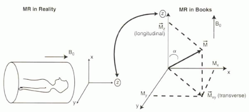 FIGURE I1-7. Orientation of magnetization in reality and in books. |
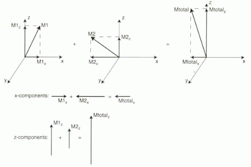 FIGURE I1-8. Vector addition in the xz plane can be accomplished by summing x and z components. |
BACKGROUND READING: Vector Addition
There are at least two different ways to perform vector addition. One is to overlay each vector from head to tail (Figures I1-4 and I1-5). For example, as shown in Figure I1-4, the vector M can be formed by the sum of Mx and Mz, laid from head to tail. Similarly, in three dimensions, the magnetization vector is the sum of Mxy and Mz (Figure I1-5).
Alternatively, vectors can be summed by adding each of their orthogonal components, Mx, My, and Mz (Figure I1-8). For example, consider two vectors in the xz plane, M1 and M2. To add these two vectors, first break each vector down into its x and z components, M1x, M1z, M2x, M2z. Then sum the x components and z components separately: Mtotalx = M1x + M2x. Mtotalz = M1z + M2z. The resulting vector Mtotal is simply the sum of the component totals, Mtotal = Mtotalx + Mtotalz.
Because vector addition is best understood by examples, the reader is referred to Figure I1-9. As illustrated in the figure, one key concept in vector addition is that vectors pointing in opposite directions cancel each other
out. Therefore, a large population of vectors that are randomly oriented, pointing in all directions, tends to sum to zero, because for every vector, there will likely be a vector pointed in the opposite direction.
out. Therefore, a large population of vectors that are randomly oriented, pointing in all directions, tends to sum to zero, because for every vector, there will likely be a vector pointed in the opposite direction.
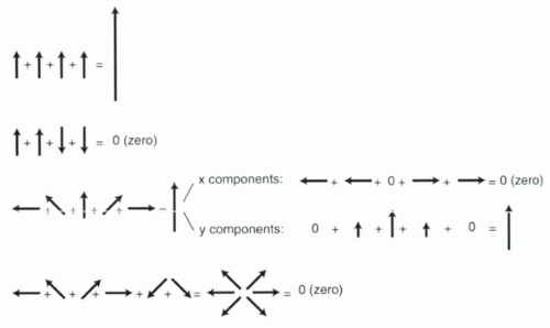 FIGURE I1-9. Examples of vector addition. In the third example, each vector is expressed in terms of its x or horizonal components (Mx) as well as its y or vertical components (My). A perfectly vertical vector has no x component; a horizontal vector has no y component. When components point in opposite directions, they cancel each other out. |
IMPORTANT CONCEPT:
When vectors are added, the components that point in opposite directions cancel each other out.
UNDERSTANDING PRECESSION AND THE LARMOR EQUATION
Precession: The Spinning Gyroscope Analogy
Outside of the MR environment, the magnetic moments of protons in the body are oriented in a completely random fashion, and therefore net magnetization is zero.
What happens when these protons are placed in a strong external magnetic field?
Two aspects of the behavior of the magnetic moments can be observed. First, the magnetic moments tend to align with the external magnetic field. They behave like tiny bar magnets exposed to a strong magnetic field and are inclined to align with it. This creates a net magnetization.
Second, a magnetic moment placed in an external field is induced to rotate around the axis of the magnetic field. To understand this movement, known as precession, consider the analogy of a wobbling gyroscope (Figure I1-10). A spinning gyroscope oriented vertically spins without any wobbling. However, once tipped off axis, gravity causes the spinning gyroscope to start to wobble. The wobbling has its own frequency (f in Figure I1-10), which can be considered independent of the frequency of spinning. The precession of protons’ magnetic moments is akin to this wobbling. In the case of the gyroscope, the wobbling frequency depends on gravity, while for protons the precessional frequency depends on the strength of the external magnetic field, B0. The precessional frequency is measured either in hertz (cycles per second, in which case it is denoted by f) or in radians per second (in which case it is denoted by ω, omega), where ω = 2πf and π (pi) is approximately 3.14.
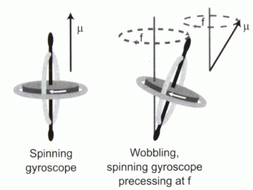 FIGURE I1-10. The wobbling, spinning gyroscope analogy for a precessing proton with magnetic moment μ. |
When exposed to the B0 magnetic field, all magnetic moments precess (or wobble) around the axis of the magnetic field. Although the magnetic moments precess at about the same frequency, they do not precess together (Figure I1-11), that is, they lack phase coherence. As a result, the transverse or Mxz components are randomly oriented. Based on the concepts of vector addition (Figure I1-9) and the very large number of protons in the tissue, transverse magnetization cancels out and is zero. Consequently, the net magnetization, M, is entirely longitudinal in the direction of B0 and stationary.
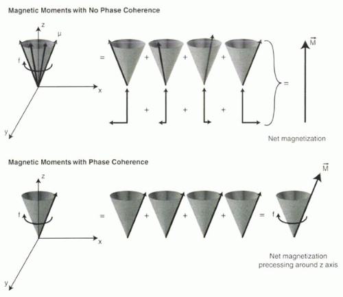 FIGURE I1-11. Precessing magnetic moments without (above) and with (below) phase coherence. When magnetic moments lack phase coherence, despite precessing at the same frequency, the transverse components in the xy plane cancel out (x components illustrated in figure), leaving only a net magnetization in the z direction. With phase coherence, the net magnetization also precesses around the z axis. |
If the magnetic moments gain phase coherence, then the net magnetization precesses around the z axis at a frequency f (Figure I1-11). In other words, net magnetization acquires a transverse component that rotates in the xy plane with a frequency f.
While vectors are useful for showing the state of magnetization at a given point in time, other tools are better for depicting the behavior of magnetization vectors over time, such as precessing magnetic moments. Sinusoidal curves can illustrate the behavior of a single magnetic moment, populations of coherent moments, as well as populations of magnetic moments that are gradually losing phase coherence. The relationship between precessing vectors and their depiction as sinusoidal curves is detailed in the following Background Reading on precessing vectors, angular frequency, and sinusoidal curves.
BACKGROUND READING: Precessing Vectors, Angular Frequency, and Sinusoidal Curves
Precessing Vectors
When placed in an external magnetic field, the magnetic moments of protons precess around the axis of that field. Because it is difficult to depict a moving magnetization vector on paper, the precessing vector is instead represented by plotting one component of the vector (usually Mx or My) against time (Figure I1-12).
CHALLENGE QUESTION: What is the value of Mx at any point in time, if φ(t) is defined as the angle between Mxy and the x axis that changes over time? What about My?
View Answer
Answer: The x component Mx changes over time and can be expressed using the cosine function (Figure I1-6 and Figure I1-13):
Mx (t) = Mxy cos φ(t)
where the angle of Mxy with respect to the x axis, φ, changes over time, as denoted φ(t). Similarly, the y component My(t) = Mxy sin φ(t).
With precessing vectors, φ is changing constantly over time. As φ changes from zero to 90° (π/2) to 180° (π) to 360° (2π) and back around the circle again, the value of Mx will also change—from Mxy to 0 to −Mxy and back to Mxy again (recall that cos 0° = 1, cos 90° = 0, cos 180° = −1, and cos 360° = 1).
The rate of change of φ per unit time is defined as an angular frequency, which is simply the precessional frequency. This frequency describes how fast
the precessing magnetic moments spin around in the xy plane, and it can be expressed using different units. The use of different units can be confusing and merits a brief discussion and explanation.
the precessing magnetic moments spin around in the xy plane, and it can be expressed using different units. The use of different units can be confusing and merits a brief discussion and explanation.
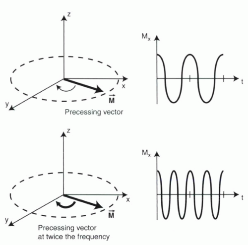 FIGURE I1-12. Precessing vectors. A precessing vector in the xy plane can be depicted in terms of its x component, Mx, over time. The frequency of precession is twice as high in the lower example, resulting in a more “compressed”-appearing sinusoidal function for Mx. |
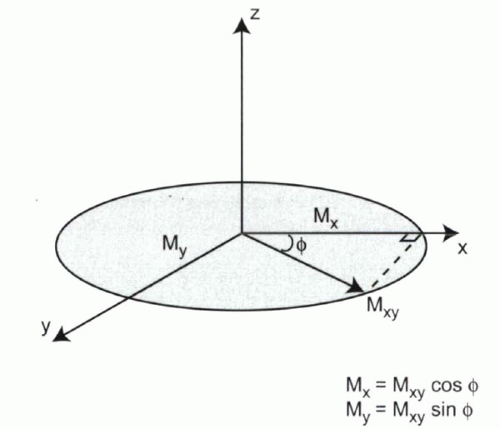 FIGURE I1-13. The x component of Mxy varies over time depending on its angle with respect to the x axis, φ. |
Angular Frequencies
A common way to express the frequency of precessing vectors is in terms of cycles per second, or the number of full 360° rotations per second. The units of hertz (Hz) are used, where 1 Hz equals one cycle per second. When frequency is expressed in these units, the symbol f is usually used for angular frequency.
Alternatively, angular frequency can be expressed in units of radians per second, where one full cycle (360°) is equal to 2π (two pi, or about 6.28) radians. This means that one cycle per second equals 2π radians per second. When angular frequency is expressed in radians per second, the symbol ω (omega) is usually used.
Both expressions of angular frequency, f and ω, are useful in MRI. In particular, ω is useful for relating frequency to the angle φ that a magnetic moment makes with the x axis. After precessing for time t, φ, in units of radians, is simply equal to the product of ω and t (ωt). Therefore, the precessional behavior of magnetization over time can be expressed in terms of Mx using the equation
Mx(t) = Mxy cos φ(t) = Mxy cos ωt
The faster the vector spins, the higher the frequency ω, and the more sinusoidal oscillations will occur per unit time. Figure I1-12 illustrates two precessing moments, one at twice the frequency of the other.
Sinusoidal Functions
There are certain properties of cosine and sine functions that are useful to understand for MR imaging. One concept is that of symmetric and asymmetric functions. Cosine is a symmetric function (Figure I1-14). This means that the cosine curve is a mirror image of itself around time = 0. In other words, cos (−ωt) = cos ωt. In contrast, sine curves are asymmetric functions: sin (−ωt) = −sin (ωt).
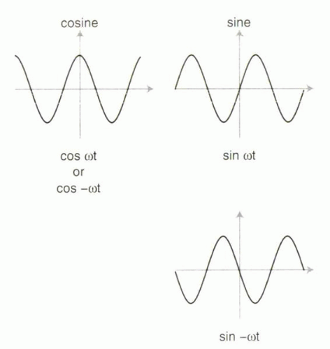 FIGURE I1-14. Symmetry of the cosine function and asymmetry of the sine function. |
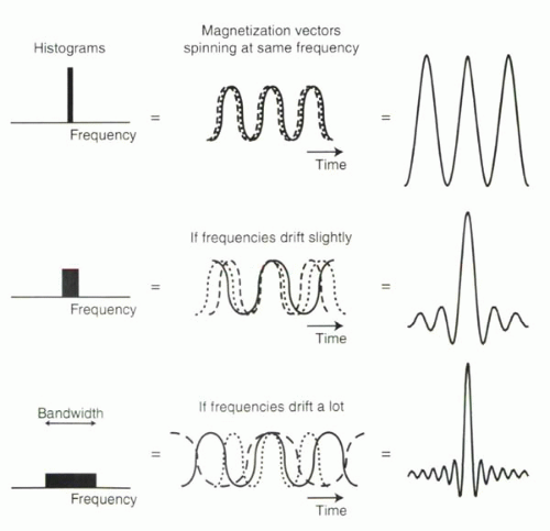 FIGURE I1-15. Transverse magnetization signal over time from many precessing magnetization vectors. With greater drifts in frequency, the net signal looks less like a sinusoidal function and more like a sinc function. |
Precessing Vectors with and without Phase Coherence
Instead of just one magnetic moment, consider what happens when there is a collection of many precessing magnetic moments.
If all the vectors precess together, then they have phase coherence. The overall amplitude of the net magnetization will be equal to the sum of the individual components, and the net magnetization will have a frequency equal to that of any individual magnetic moment (Figure I1-15, top).
What happens if the frequencies of the individual components are slightly different? They lose phase coherence and no longer precess together. Then the net magnetization curve will resemble that shown in the lower two parts of Figure I1-15. As the magnetic moments drift in frequency, the sinusoidal functions no longer sum in a straightforward way. At a reference time point (the midpoint of the curves plotted in Figure I1-15), the magnetization adds. However, away from this point, signal from magnetization vectors precessing at different frequencies cancels partly, resulting in attenuation of the signal away from the midpoint.
The resulting magnetization sinusoidal curve begins to take on the shape of a sinc function. Mathematically, a sinc function can be expressed as
sinc x = (sin x)/x (and sinc = 1 for x = 0)
As illustrated in the figure, there is a relationship between the range of frequencies and the appearance of the resulting signal. Specifically, the greater the drift in the frequencies or the wider the range of frequencies used to form the sinc function, the more “compressed” the curve appears (Figure I1-15). The extreme frequency contributions result in the narrowing of the summed signal and its side ripples.
The Larmor Frequency and the Larmor Equation
One of the most important concepts of MR physics is the Larmor equation, which describes the relationship between the precessional frequency and the external magnetic field to which the protons are exposed.
The Larmor equation says that the angular frequency at which the magnetic moments precess around the axis of the magnetic field, called the Larmor frequency, is proportional to the strength of the magnetic field. The higher the field strength, the faster the precession,
f = γB
where f = precessional frequency, B is the magnetic field strength, and γ (gamma) is the gyromagnetic ratio. γ depends on the type of nucleus being imaged. For hydrogen protons, γ ≅ 42.6 megahertz per tesla (MHz/T; recall that a frequency denoted f is measured in cycles per second, or hertz, and 1 MHz = 1 million cycles per second). Compared to other nuclei, hydrogen protons have a large gyromagnetic ratio. This, in addition to their natural abundance, makes hydrogen ideal for MR imaging because small changes in the magnetic field cause large, and readily measurable, changes in signal. For a 1.5 T magnet, the Larmor frequency is
or about 64 million cycles per second. If the magnetic field were uniformly and perfectly 1.5 T throughout, then all protons in the magnet’s bore would precess around the z axis at the same frequency of about 64 MHz.
 |
IMPORTANT CONCEPT:
The Larmor equation states that the frequency of precession of magnetic moments around the axis of an external magnetic field, called the Larmor frequency, is proportional to the strength of the magnetic field.
As will be discussed later, no MRI system has a perfectly homogeneous magnetic field, B0, throughout its bore. What then is the effect of heterogeneity in the magnetic field? The answer lies simply in understanding the Larmor equation: Protons that are exposed to slightly different magnetic fields will precess at slightly different frequencies. More specifically, protons that are exposed to fields less than 1.5 T will precess slightly more slowly than those exposed to 1.5 T, while those exposed to fields greater than 1.5 T will precess more quickly.
Frequency and Phase
In MRI, the effects of magnetic field differences on the precessing of protons are characterized in terms of frequency and phase. Frequency is the rate of change of phase. It is described simply as the number of cycles (or millions of cycles) per second. By the Larmor equation, frequency changes directly in proportion to the strength of the magnetic field.
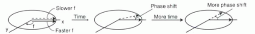
What about phase? Phase refers to the orientation of one magnetization vector relative to some reference. It can be thought of as the angle between two vectors or between a vector and a reference axis, for example the angle φ between a vector Mxy and the x axis (Figure I1-13). If two protons start in the same position but precess at different frequencies, then with time the protons will be out of phase; that is, there will be a phase difference between them. The greater the frequency difference between two protons, the greater the phase difference over a given time. For a given difference in frequencies, the more time elapsed, the greater the phase difference separating the two protons. However, phase shift is uniquely defined only across a range of 360°. When a phase shift exceeds 360° (say, 370°), it becomes indistinguishable from a phase shift 360° less (say, 10°). Nevertheless, the cumulative phase difference between two protons precessing at two frequencies is proportional to the difference in frequencies and to the duration of time that has passed (Figure I1-16).
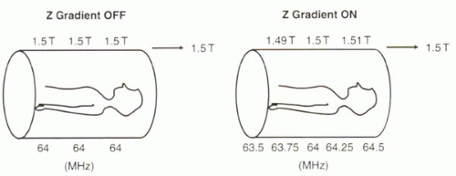 FIGURE I1-17. Varying the magnetic field with a z gradient alters the precessional frequencies of protons along the z direction. |
IMPORTANT CONCEPT:
Protons exposed to different magnetic fields will precess at different frequencies. Consequently, phase differences will progressively accumulate between their magnetic moments.
Gradients
Precessional frequencies can be deliberately made to vary with position in the magnetic field by applying a magnetic field gradient along a given direction. A magnetic field gradient refers to a magnetic field that varies in a certain direction (Figure I1-17). In the setting of a gradient, the precessional frequencies of protons vary spatially in a predictable fashion. For example, with a linear magnetic field gradient in the z direction (Figure I1-17), the field toward the subject’s feet is slightly weaker than 1.5 T, while the field toward the head is slightly stronger. The protons at the feet therefore precess more slowly than the middle of the body, and those in the head precess more quickly. For a given linear magnetic field gradient, the range of precessional frequencies across the field of view, Δf, or the bandwidth, can be predicted using the Larmor equation,
Δf = γΔB
where ΔB is the range of magnetic field strengths across relevant region.
IMPORTANT CONCEPT:
Magnetic field gradients cause precessional frequencies to vary spatially in a predictable fashion, according to the Larmor equation.
Spatial variation of the external magnetic field causes a corresponding variation in Larmor frequencies for the magnetic moments exposed to the gradient. What would the effect of deliberately varying precessional frequencies have on the net magnetization? Based on the previous Background Reading (Figure I1-15), the cumulative signal from protons exposed to a linear magnetic field gradient will resemble a sinc function (Figure I1-18).
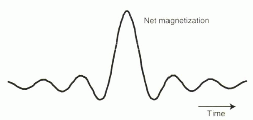 FIGURE I1-18. The composite signal from protons exposed to a magnetic field gradient resembles a sinc function. |
Fat versus Water
So far, the discussion about the Larmor frequency has assumed that all hydrogen nuclei are alike, but they are not. The molecular environment experienced by a given hydrogen proton is not exactly equal to B0


Stay updated, free articles. Join our Telegram channel
Full access? Get Clinical Tree
