k-Space
k-space is the name of the place where MR echoes are stored. As introduced in Chapter I-1, one of the miracles of MRI is that k-space turns out to be the Fourier transformation of the original tissue slice. Because of the duality property (as discussed in Chapter I-1), taking the Fourier transformation of k-space then gives back a representation of the tissue slice, called the MR image (Figure I6-1).
So far, the pulse sequence diagram has been explained with the sole purpose of addressing spatial localization. To grasp many of the more advanced concepts in MR physics, a more profound understanding of k-space and its relationship with the pulse sequence diagram is necessary. This chapter focuses on how the application of the gradients described in the pulse sequence diagram produces echoes that represent the Fourier transform of the tissue slice. With this knowledge, more innovative and complex ways of filling k-space can be explored. Combined with a greater understanding of the relationship between k-space and the image discussed in Chapter I-7, the reader will then be equipped to understand the fast imaging techniques that are commonly used in cardiovascular MRI, the “k-space shortcuts,” to be presented in Chapter I-8.
KEY CONCEPTS
[right half black circle] k-space is the Fourier transformation of the tissue slice and of the MR image.
[right half black circle] A simplified version of the Fourier transformation H(kx, ky) of an image h(x, y) can be expressed in terms of its mathematical formula,  .
.
.[right half black circle] Gradient-induced phase shifts can be represented as a sinusoidal modulation of the phases of magnetization vectors. The modulation can be expressed as cos kxx or cos kyy, where kx and ky are proportional to the areas under the gradient waveforms, Gx and Gy, respectively. During application of a gradient, such as Gx, the value of kx changes continuously, since kx is proportional to Gx × t.
[right half black circle] Application of gradients and summation of signal using receiver coils effectively generate the Fourier transform of an image.
[right half black circle] Pulse sequence diagrams describe the recipe for generating an MR image in terms of the k-space trajectory.
[right half black circle] To improve the efficiency of a k-space trajectory, portions that do not involve data sampling should be traversed as rapidly as possible.
[right half black circle] k-space trajectories can be designed to suit different demands for efficiency and image quality.
WHAT IS k-SPACE?
In this chapter, k-space is defined as the Fourier transform of the tissue slice or the MR image. The reader is encouraged to review the part in Chapter I-1 on Fourier transformations and, in particular, Figures I1-28 and I1-29, for a qualitative understanding of Fourier transforms as spatial frequency maps. This section presents a more quantitative definition of the Fourier transformation.
In two dimensions, the Fourier transform H(kx,ky) of an image h(x,y) can be expressed as
This equation describes how to obtain the Fourier transform of an image. (Strictly speaking, the full form of the Fourier transform is
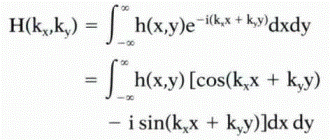
where i is the imaginary number  . The sine term has imaginary values and is ignored in this book to simplify the equation.) Before the meaning and implications of this equation are explored, the terms h(x,y) and H(kx,ky) must be explained in greater detail.
. The sine term has imaginary values and is ignored in this book to simplify the equation.) Before the meaning and implications of this equation are explored, the terms h(x,y) and H(kx,ky) must be explained in greater detail.The expression h(x, y) refers to the spatial distribution of signal intensities in an image, for example, a tissue slice
or an MR image. Either can be thought of as a grid or array of numbers, where at each pair of coordinates in the array, (x,y), the value of the intensity at that location has a value equal to h(x,y). In the case of an MR image, the intensity values at each location h(x,y) depends on the interplay between intrinsic tissue properties such as T1 and T2 relaxation times and MR pulse sequence parameters such as TR, TE, and flip angle. The coordinates of the image space, h(x,y), are usually centered at location (x,y) = (0,0), so that for a 256 × 256 matrix image, x values would range from −127 to +128, and y values would also range from − 127 to + 128 (Figure I6-2). Based on the size of each voxel, x and y can also be expressed in units of distance (cm, for example).
or an MR image. Either can be thought of as a grid or array of numbers, where at each pair of coordinates in the array, (x,y), the value of the intensity at that location has a value equal to h(x,y). In the case of an MR image, the intensity values at each location h(x,y) depends on the interplay between intrinsic tissue properties such as T1 and T2 relaxation times and MR pulse sequence parameters such as TR, TE, and flip angle. The coordinates of the image space, h(x,y), are usually centered at location (x,y) = (0,0), so that for a 256 × 256 matrix image, x values would range from −127 to +128, and y values would also range from − 127 to + 128 (Figure I6-2). Based on the size of each voxel, x and y can also be expressed in units of distance (cm, for example).
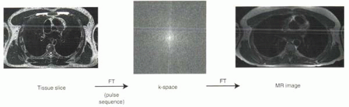 FIGURE I6-1. k-space. MR image generation involves filling k-space with the intensities of measured echoes, followed by a Fourier transformation that recreates an image representation of the original tissue slice. (Note that, as discussed in Chapter I-1, for simplicity, the Fourier transformation and inverse Fourier transformation are considered identical.) |
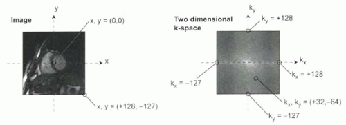 |
The expression for k-space, H(kx,ky), similarly refers to a grid or array of numbers (Figure I6-2). The coordinates in k-space are defined in terms of (kx, ky), where kx corresponds to the spatial frequency cos kxx and ky the spatial frequency cos kyy. The units of the spatial frequencies, kx and ky, are usually given in inverse distance (1/cm or cycles per cm). At each coordinate in the grid, the value of the intensity at that point equals H(kx,ky) and reflects how much of the spatial frequency component, cos(kxx + kyy), is contained in the image. The coordinates of k-space are usually centered at location (kx,ky) = (0,0), so that for a 256 × 256 k-space matrix, kx would range from −127 to + 128 and ky also from −127 to + 128 (Figure I6-2).
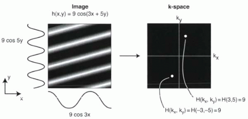
To illustrate the relationship between h(x, y) and H(kx,ky), consider the image of a wavy potato chip or piece of corrugated cardboard tilted off axis depicted in Figure I6-3. Mathematically, this image can be defined by the following function:
h(x, y) = 9 cos (3x + 5y)
which means that the value of the intensity of the image at every location (x,y) can be calculated by plugging in values of x and y into the expression 9 cos (3x + 5y).
To derive the Fourier transformation or spatial frequency map of this image, observe that the overall spatial variation in the image is defined simply as cos (3x + 5y). This means that the only spatial frequency that is needed to describe this function has kx = 3 and ky = 5. That is, the Fourier transformation has only a spike at one location, (kx,ky) = (3,5). The value of H(kx,ky) at that location, H(3,5), would be equal to the amplitude of the sinusoidal
function in the image, which reflects how high the peaks and deep the grooves are in the surface. In the example, the amplitude is 9, and therefore H(kx, ky) = H(3, 5) = 9. Note that because of the symmetry of cosine functions (cos(−x) = cosx), there is another nonzero value in k-space at (−3,−5), as shown in Figure I6-3.
function in the image, which reflects how high the peaks and deep the grooves are in the surface. In the example, the amplitude is 9, and therefore H(kx, ky) = H(3, 5) = 9. Note that because of the symmetry of cosine functions (cos(−x) = cosx), there is another nonzero value in k-space at (−3,−5), as shown in Figure I6-3.
 |
In the Fourier transform equation, the integral sign,  , indicates that the expression between the
  and the dx dy should be summed for all values of x and y. Therefore, the equation says that the value of the Fourier transform, H(kx,ky), of an image, h(x,y) can be calculated by multiplying each intensity value in the image by a sinusoidal function, cos (kxx + kyy), and then taking the integral for all values of x and y.
, indicates that the expression between the and the dx dy should be summed for all values of x and y. Therefore, the equation says that the value of the Fourier transform, H(kx,ky), of an image, h(x,y) can be calculated by multiplying each intensity value in the image by a sinusoidal function, cos (kxx + kyy), and then taking the integral for all values of x and y.Translated into words, this equation says that to determine the value of k-space at a particular frequency, kx, ky, the image must be multiplied by cos(kxx + kyy) and then summed up for all values x and y across the entire image.
The next section will show how the gradients and receiver coil are used to perform the calculation.
IMPORTANT CONCEPT:
By definition, the value of k-space at a particular kx, ky can be determined by performing two steps: (1) multiplying the image by cos(kxx + kyy) and then (2) summing the value of all the signal across the entire image.
HOW AN MR PULSE SEQUENCE CONVERTS A TISSUE SLICE INTO ITS FOURIER TRANSFORM (k-SPACE)
There are two steps to getting the Fourier transform of a tissue slice, that is, k-space. The first step is to apply frequency– and phase-encoding gradients. The second step is to use the receiver coil to collect all of the signal across the tissue slice, that is, to sum up all the signal from all the protons in the slice. This section will show how applying gradients effectively multiplies the image by cosine functions and how the receiver coil essentially integrates or sums the resulting product.
Application of a Gradient = Multiplying the Image by a Cosine Function
With the application of a linear gradient across the field of view, the varying magnetic field strength causes protons to precess at different frequencies, and consequently a phase shift across protons accumulates. As illustrated in Figure I6-4, phase shifts can be expressed as a sinusoidal modulation of the phases, so that the effect of a gradient can be seen as multiplying the original magnetization vectors by a cosine function along the direction of the gradient. In Figure I6-4, the gradient induces a phase shift of 720° along the column of tissue. The resulting pattern of magnetization vectors is simply equal to the original magnetization vectors multiplied by the function, cos 2y. Note that the amplitudes of the magnetization vectors reflect the relationship between tissue properties and MR pulse sequence parameters and are unaffected by the gradient. Only their orientations or directions are modulated.
For the purposes of translating this concept into an understanding of k-space, the frequency of the sinusoidal change in phase is called “k.” For example, in Figure I6-4, ky = 2.
The longer the gradient stays on, the greater phase dispersion. Initially, the phase shifts will be slight, corresponding to a low-frequency cosine modulation of phases. If the gradient is strong, then the phase shifts will increase more quickly over time (Figure I6-5). Translated in terms of k, which is defined as the frequency of the sinusoidal function that is induced by the gradients, the longer the gradient is left on, the larger the k. The stronger the gradient, the faster k will increase.
CHALLENGE QUESTION: What is the effect of applying no phase-encoding gradient?
View Answer
Answer: Multiplying cos Oy or cos 0 is the equivalent to multiplying by 1. (Recall from Chapter I-1 that cos 0 equals 1.) This reflects the
fact that magnetic moments retain their original magnitude and phase with zero phase-encoding gradient.
fact that magnetic moments retain their original magnitude and phase with zero phase-encoding gradient.
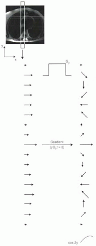 FIGURE I6-4. Gradients induce a sinusoidal phase shift. For example, a gradient in the y direction that causes phase shift of 720° (two full cycles of 360°) has the effect of multiplying the original magnetization vectors by cos 2y. The magnitudes of the vectors along the column of tissue vary according to the signal intensities of the tissues. |
IMPORTANT CONCEPT:
Gradients cause dephasing. The gradient-induced phase shifts can be represented as a sinusoidal modulation in phase. The stronger the gradient and the longer its duration, the greater the sinusoidal variation.
The observations about gradients in the y direction also hold true for gradients in the x direction. With Gx, the dephasing across the x direction can be expressed as the original magnetic moments being multiplied by cos kxx, where the coefficient kx describes the sinusoidal variation of the cosine function in the x direction. kx will progressively increase the longer the gradient Gx is left on.
kx,y Proportional to the Area under the Gx,y Gradient Curve
As discussed in Chapter I-4 (Figure I4-3), the amount of dephasing caused by a gradient is proportional to the area under the gradient curve. The gradient pulse is of constant strength, described by its strength, G, and has duration, t. The net effect of any gradient is G × t.
In this chapter, dephasing is expressed more specifically in mathematical terms as a multiplication of the original signal by a sinusoidal function, cos kxx or cos kyy, where the coefficients, kx and ky, represent the frequency of the sinusoidal modulation. It follows that, as measures of dephasing, kx and ky are proportional to the areas under their respective gradient curves (Figure I6-6):
kx = Gx × t × γ
ky = Gy × t × γ
Each gradient acts independently by modulating the dephasing in different directions. The gradients can be applied simultaneously or sequentially. Gradients can have reversed polarity and cause phase shifts that are reversed in direction, corresponding to negative values of k. With negative gradients, the stronger the negative gradient, the more negative the k values.
The Elusive, Ever-Changing k
While a gradient is on, the dephasing is cumulative, and k values (kx or ky) will continuously change. When the gradient is positive, k progressively increases over time. When the gradient is negative, k progressively decreases. When the gradient is turned off, the phase differences are maintained because the protons return to precessing at
the same 64 MHz frequency. Given that their phase dispersion stays the same, k maintains the same value it had at the instant the gradient was turned off.
the same 64 MHz frequency. Given that their phase dispersion stays the same, k maintains the same value it had at the instant the gradient was turned off.
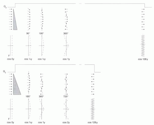 FIGURE I6-5. Gradients and sindusoidal modulation of phase shifts. Phase shifts can be represented as the original magnetic moments multiplied by a sinusoidal function whose frequency increases as the gradient strength and duration increase. Using a gradient that is twice as strong, the maximum phase shift is achieved in half the time (below). As depicted in Figure I6-4, the magnetic moments will vary in amplitude, depending on properties such as proton density, T1 relaxation, and T2 relaxation. For simplicity these variations are ignored. |
IMPORTANT CONCEPT:
The dephasing effect of a gradient is equivalent to modulating the phase by a sinusoidal function, cos kxx or cos kyy, where kx and ky are proportional to the area under the gradient waveforms, Gx and Gy, respectively. While a gradient such as Gx is on, the value of kx changes continuously, because kx is proportional to Gx × t.
Integration by the Receiver Coil
During the readout period, as the echo is being formed, data are collected by the receiver coil. The measured signal depends on the cumulative contributions of all protons in the field. The coil effectively sums all signals from all protons.
The signals being emitted by the protons represent the magnetization vectors modulated by the sinusoidal function induced by the gradients. Therefore, when the receiver coil records signal, it is equivalent to measuring the sum of signals from the original tissue multiplied by a cosine function. These words ring some bells. They are the definition of the Fourier transform!
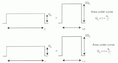 FIGURE I6-6. Relationship between gradients and the resulting sinusoidal modulation of the signal by cos kxx or cos kyy. The frequency of the sinusoidal modulation of phase is proportional to the area under the gradient curve, which depends on its amplitude and duration. |
Summary: Gradients + Receiver Coil = Fourier Transform
Stay updated, free articles. Join our Telegram channel

Full access? Get Clinical Tree


