Flow
Blood flow can create different kinds of effects on MR images. Some are highly desirable and can be used to image vessels, while others are undesirable and lead to artifacts. This chapter introduces a few basic principles of blood flow in the body. Then the different kinds of effects that flow has on MR images are reviewed. Chapter II-1 concludes by discussing artifacts and ways to minimize them. The specifics of vascular MR sequences, such as time-of-flight imaging (Chapter II-2), phase–contrast angiography and flow quantification (Chapter II-3), and gadolinium-enhanced MR angiography (Chapter II-4), are considered in subsequent chapters.
KEY CONCEPTS
[right half black circle] Flow patterns vary depending on vessel geometry and contour.
[right half black circle] Flow can cause signal loss or signal gain on both spin echo and gradient echo sequences.
[right half black circle] Spin echo sequences are typically used for black-blood imaging; parameters that favor signal loss due to flow include a longer TE and thin slices oriented perpendicular to flow.
[right half black circle] Gradient echo sequences are often used for bright-blood imaging; flow-related enhancement is maximized with a longer TR and thin slices oriented perpendicular to flow.
[right half black circle] Flow-related dephasing can be reduced by minimizing TE or by using flow compensation (gradient moment nulling), which requires longer TE.
[right half black circle] Artifacts related to flow include pulsation artifacts and overestimation of stenoses.
BLOOD FLOW IN VESSELS
Types of Flow
The study of blood flow in the vessels of the body is a vast and complex topic. The behavior of blood depends upon several factors, including its velocity and geometry of the vessels. In long, large, widely patent vessels, the flow usually can be described as laminar flow. The velocity profile across the vessel is parabolic—negligible velocity at the wall (Figure II1-1) and maximum velocity in the center. With laminar flow, the maximum velocity is equal to twice the average velocity across the vessel.
At the entrance of an aortic branch vessel such as the renal artery, the flow across the orifice starts as plug flow, that is, the velocity across the entire vessel is constant. With plug flow, the maximum velocity and mean velocity are identical.
A stenosis within a vessel causes blood to flow at high velocities through the narrowing. Beyond it, flow is nonlaminar, with vortices or eddies, reflecting turbulent flow. Turbulent flow causes signal dephasing in MR and contributes to an overestimation of vessel stenosis. Some distance beyond turbulent flow, the flow regains laminar behavior (Figure II1-1).
One special consideration in blood flow is what happens at vessel bifurcations, such as the bifurcation of the common carotid artery into the internal and external carotid arteries (Figure II1-1). As a consequence of flow separation, the laminar flow is disturbed in the branches, and small vortices may form. On MR imaging, these areas can cause signal loss and be misinterpreted as areas of vessel stenosis even in the absence of disease. These areas are challenging because regions of flow separation are prone to the formation of atherosclerotic plaque. Flow is further disturbed in the setting of stenoses, thereby worsening the signal loss.
Measures of Flow
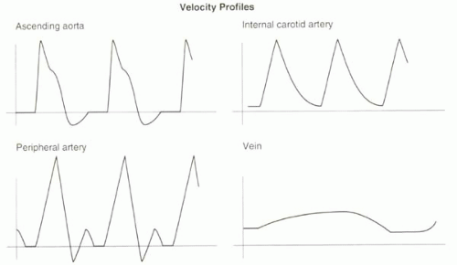
By definition, the velocity of blood is the distance traveled per unit time (typically in units of centimeters/sec or meters/sec). In general, the velocity of blood in a vessel is not uniform across its lumen. The maximum velocity is typically near the center of the vessel, while slower velocities are measured toward the vessel wall (Figure II1-1). In addition to the spatial variation, arterial flow in the body is pulsatile, with a period defined by the cardiac cycle.
Velocities change over time, typically higher during systole and lower during diastole. One of the most commonly used measurements of velocity in the clinical setting is the absolute maximum velocity, also known as the peak systolic velocity, which represents the highest velocity across the vessel cross section during peak systolic flow.
Velocities change over time, typically higher during systole and lower during diastole. One of the most commonly used measurements of velocity in the clinical setting is the absolute maximum velocity, also known as the peak systolic velocity, which represents the highest velocity across the vessel cross section during peak systolic flow.
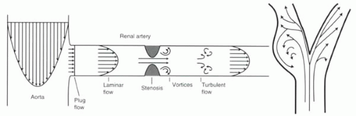 FIGURE II1-1. Flow patterns illustrated in the aorta and renal artery, including a renal artery stenosis (left), and in the carotid bifurcation (right). |
Velocity is commonly called “first-order flow.” What are referred to as “higher-order” flow patterns include acceleration and jerk. Acceleration (“second-order flow”) is defined as a constant change in velocity over time. Jerk (“third-order flow”) is a constant change in acceleration over time. Because of the complex geometry of vessels, combined with the pulsatility of blood, flow in most vessels can be characterized as including higher-order flows. However, for many applications of MR, constant velocities are assumed.
Blood flow, or flow rate, on the other hand, refers to the volume of blood moving through a vessel in a given time (typical units of mL/sec or mL/min). Typically, with MRI, instantaneous flow is measured by assuming a constant velocity of blood over a short measurement period. To determine the instantaneous flow rate in a vessel, the average luminal velocity of blood at that time (cm/sec) is multiplied by the cross-sectional area of the vessel (cm2):
Often the total average flow over a specified period, such as one heartbeat, is reported. Examples of useful flow measurements include the measurement of total flow through the ascending aorta per heart beat (as a measurement of stroke volume) and the determination of intracardiac shunt fractions by comparing flow rates through the ascending aorta and main pulmonary artery. These are usually calculated by determining the average luminal velocity over one heartbeat and multiplying it by the cross-sectional area.
[right half black circle] TABLE II1-1 Typical peak velocities of blood in normal vessels | ||||||||||||
|---|---|---|---|---|---|---|---|---|---|---|---|---|
|
IMPORTANT CONCEPT:
Flow patterns in blood vessels vary depending on vessel geometry and the presence of pathology such as atherosclerotic plaque.
Typical velocities
Normal peak velocities of blood in different vessels of the body are listed in Table II1-1.
Arterial blood flow is pulsatile, and therefore velocities vary considerably across the cardiac cycle (Figure II1-2). The thoracic aorta normally has a large diastolic flow reversal that is equivalent to approximately 15% of the forward flow; the reversal is responsible for diastolic filling of the coronary arteries. In the peripheral arteries, a triphasic velocity waveform is normally seen, caused by the relationship between the pulsatility of blood, the distensibility of vessel walls, and the high resistance to circulation of the distal vessels in the musculature. In the setting of arterial stenosis, measured velocities can greatly exceed values given in Table II1-1. When stenoses become nearly occlusive, velocities decrease.
In the venous system, the flow is nearly constant except for mild variations related to breathing where intrathoracic pressure changes affect venous return.
Types of Flow Effects
Flow can cause signal gain or signal loss depending on the nature of the pulse sequence and the nature of the flow (Table II1-2). Both effects are exploited in MR imaging. Techniques that rely on signal loss or signal void are referred to as black-blood imaging methods. Those that maximize flow-related enhancement are called bright-blood imaging techniques. It is important to understand the different causes of signal gain and loss so that each approach can be designed to minimize the factors that cause the opposite effect. Additionally, an understanding of these relationships can help avoid errors in interpretation that may arise from unintended flow-related effects. In the following sections, each flow effect is described first, then the concepts are synthesized in a discussion on how to perform bright-blood or black-blood MR angiography (MRA).
FLOW-RELATED SIGNAL LOSS
Flow Voids on Spin Echo
The loss of signal in moving blood on spin echo imaging has given rise to the alternative term used to describe spin echo imaging in the heart and vessels: “black-blood” imaging. The signal loss occurs because to generate a spin echo, protons must experience both the 90° and 180° pulses, both of which are typically slice selective. Blood that moves quickly through the slice of interest will not experience both RF pulses and therefore will not generate any signal (Figure II1-3).
|
Whether a complete signal void is produced by moving blood depends on the slice thickness and the time between the 90° and 180° pulses, or TE/2. Blood that traverses the slice thickness in the time TE/2 will not see both pulses. The minimum velocity needed to generate a signal void, Vvoid, is therefore

Conditions favorable for generating a signal void are thinner slices and longer TE.
For example, if the slice thickness is 5 mm and the TE is 50 msec in a spin echo sequence, then the minimum velocity for complete signal void is
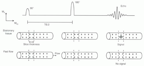 FIGURE II1-3. Effect of flowing blood on spin echo generation. Small arrows within the vessels indicate the net magnetization of protons in the blood. Only protons that are tipped into the transverse plane by the 90° pulse and then refocused within the transverse plane by the 180° pulse can generate an echo. |
However, if the slice thickness is 10 mm, then the minimum velocity for a signal void is
From Table II1-1, for a 5 mm slice, Vvoid is sufficiently low to ensure that almost all vessels, including all arteries and most veins, will demonstrate complete signal void on this sequence provided the images are gated to systole. Note that with a thicker slice, veins may have some visible signal intensity.
A sequence with a longer TE is more likely to generate a signal void than a sequence with short TE because there is more time for the blood to flow out of the slice during the pulse sequence.
Because blood flow is pulsatile, the timing of the acquisition relative to the cardiac cycle impacts the MR signal. Flow voids are greater in systole and less in diastole. Additionally, if images are acquired in the plane of flow rather than perpendicular to it, some protons, despite rapid flow, may still experience both 90° and 180° pulses. Complex patterns of signal intensity may result.
View Answer
Answer: As discussed in Chapter I-9, double inversion recovery prepulses can be used to null signal from blood.
Flow-Related Dephasing (Spin Echo and Gradient Echo)
One recurring theme in MR physics is that gradients cause dephasing. To compensate for dephasing, most gradients are applied in two parts: a dephasing lobe and a rephasing lobe. When the area under the dephasing lobe equals the area under the rephasing lobe, protons are assumed to be in phase.
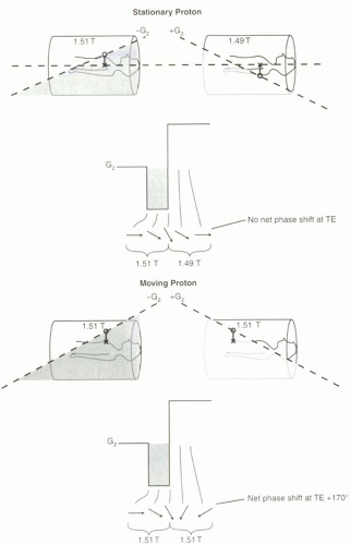
One assumption that has been implicit in these discussions is that the protons are stationary in the magnetic field. That is, for the rephasing lobe to cancel out the effects of the dephasing lobe, the protons must stay in the same location for each gradient. Protons that experience a stronger magnetic field than 1.5 T during dephasing gradient will experience a weaker magnetic field than 1.5 T during the rephasing gradient, and vice versa.
But what if protons are moving?
If protons are moving along the direction of the frequency-encoding gradient, then they will not necessarily experience dephasing and rephasing in the manner intended. That is, the dephasing will not equal the rephasing. In fact, moving protons will accumulate a net phase
shift relative to stationary protons that is dependent on their velocity and direction. Figure II1-4 illustrates two scenarios—stationary versus moving protons—in a gradient echo pulse sequence. In this example, if a proton moves from the head to the feet (arterial flow), the net phase shift will be positive, while a proton moving in the opposite direction (venous flow) will accumulate a negative net phase shift. The gradients shown are Gz, but the same principles apply to gradients in any direction, and most often refer to those in the readout direction (Gx).
shift relative to stationary protons that is dependent on their velocity and direction. Figure II1-4 illustrates two scenarios—stationary versus moving protons—in a gradient echo pulse sequence. In this example, if a proton moves from the head to the feet (arterial flow), the net phase shift will be positive, while a proton moving in the opposite direction (venous flow) will accumulate a negative net phase shift. The gradients shown are Gz, but the same principles apply to gradients in any direction, and most often refer to those in the readout direction (Gx).
 Get Clinical Tree app for offline access 
|


