Of the clinical uses for EEG in the management of epilepsy, localization of the epileptogenic focus is perhaps second in importance only to diagnosis. This is particularly true for those patients with medically uncontrolled, partial seizures, who may be surgical candidates. However, EEG analysis in most clinical epilepsy centers begins and ends with the visual inspection of EEG traces. Localization of spike and seizure sources is based on identifying the electrode(s) recording the most prominent negative potential or clearest negative rhythm, that is, the scalp negative field maximum. Little, if any, attention is paid to the presence or location of any associated positive field. This simplistic form of source localization is based on several false assumptions, namely, that the cortical generator underlies the negative field maximum, that a discrete source must produce a focal scalp potential, and that a widespread potential means a diffuse or multiple sources. Unfortunately, none of these assumptions are necessarily true.

Scalp EEG contains much more spatial and temporal information than can be appreciated by eye. This information is now easily extracted by modern computer-assisted analysis techniques. This chapter will review the use of voltage topography and dipole source modeling in the characterization and localization of epileptiform spike and seizure potentials. Dipole source modeling is an advanced method of analyzing and interpreting EEG data. It is based, however, on simple principles that need to be understood before the technique can be fully appreciated. In reality, the EEG is a time series of continually changing voltage fields of differing polarity and magnitude over the surface of the head. The EEG as most know it, namely, traces of voltage potential difference over time between electrodes, is simply a creation of measurement and display techniques. It is important to think of EEG as voltage fields and not simply as lines on a display. This is because the contours of these fields and the location and amplitude of negative and positive field maxima convey all the information that is necessary for proper source localization. With the advent of digital EEG and advanced computer techniques, localization of epileptogenic foci is easily transformed from an art form into a science.

EEG SPIKE AND SEIZURE SOURCES

In order to model the cortical generators of EEG accurately and interpret the results of such modeling, you must know the typical characteristics of such sources. For example, what is the average size or range of sizes of cortical sources that produce typical scalp EEG potentials? Unfortunately, there have been few studies to determine these directly and in vivo. As reviewed in Chapter 2, the widely quoted study by Cooper et al (1), which identified 6 cm² as the minimal area of a cortical source resulting in a scalp EEG potential, was in fact an in vitro experiment using a fresh piece of cadaver skull. Only simultaneous scalp and intracranial EEG recording affords the opportunity for direct validation.

Those who have evaluated patients with intracranial electrodes for possible epilepsy surgery have known for some time that patients have far more ECoG spikes than scalp EEG spikes. Thus, much of the activity recorded from invasive electrodes is not visible from the scalp. A number of years ago, informal observations with simultaneous scalp and intracranial EEG in epilepsy patients suggested that cortical sources of typical EEG spikes and seizure rhythms were much larger than anticipated, sometimes exceeding 30 cm² of gyral area (2,3). More recently, a rigorous investigation, again with simultaneous scalp and cerebral recordings, confirmed that 6 cm² is too small for the minimal source area (4). Rather, 10 cm² of synchronously active cortex is usually necessary to produce a recognizable scalp potential, and most prominent EEG spikes have source areas two to three times greater (see Figs. 2.4 and 2.5 in Chapter 2). Thus, the actual sources of scalp-recognizable epileptiform potentials are not discrete, but rather they are sublobar at a minimum.

Accordingly, this extended size for cortical foci must be taken into consideration when interpreting dipole and other source models of epileptiform potentials. Concerns for millimeter accuracy when dealing with epileptic foci thus make little sense because the actual cortical sources are multiple square centimeters in size. Similarly, resolving two or more theoretical sources a few millimeters apart in simulation studies is again hardly pertinent in the clinical arena, given the extended nature of real cortical generators of scalp EEG. This does not mean that discrete source models, such as dipoles, cannot be useful even though they do not accurately depict source area. It just means that they have to be interpreted properly.

CORTICAL SOURCE FACTORS AND SCALP EEG POTENTIALS

There are several properties of cortical sources that are influential in determining the character of the scalp EEG field produced. They can be divided into physical factors (location, area, orientation) and functional factors (amplitude, frequency, synchrony). Some are self-evident, such as source location and activity amplitude, while others are less obvious. Source area has been discussed in Chapter 2 and is critical. Most cerebral potentials are not recordable at the scalp because of insufficient source area, rather than source depth or activity amplitude. Source orientation is also a significant factor that is less well appreciated.

Being quite extended, spike and seizure sources typically involve several lobar gyri and sulci. Although cortical convolutional geometry may be complex, fields produced by opposing walls of sulci will typically cancel each other. Voltage fields from unopposed gyral crowns tend to predominate in any resultant scalp field. A reasonable simplifying assumption is that spike and seizure scalp EEG fields appear as though arising from a smooth, lissencephalic brain, with only the major invaginating fissures exerting a significant influence. Although usually curved, the patch of the cortex activated in a cortical spike has some net orientation. The orientation of the voltage field of a spike from a given location is orthogonal to the surface orientation of that cortex. Thinking about it in another way, it is the same as the average orientation of the pyramidal cells in that cortical patch. Depending on the net orientation of the cortical source, the resultant EEG field may be radial, oblique, or tangential to the skull surface (Fig. 12.1). Only in the case of a radial source will the field maximum be directly above it. In all other cases, the field maxima will be displaced to either side of the source. In the case of truly tangential sources, the negative and positive field maxima will be equally displaced on either side of the source, and directly above the source no potential will be recordable. Thus, assuming that the location of an epileptic focus is directly under the electrode, recording the maximal potential can be dangerously inaccurate.

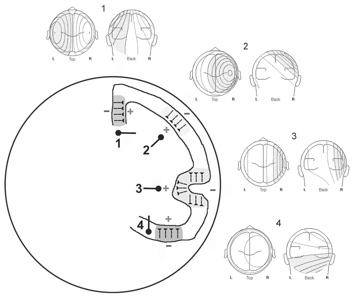
Figure 12.1: Example cortical sources 1 to 4 depicted in a schematic head/brain in coronal cross section. Typical pyramidal cell orientations are shown for each source. Resultant scalp voltage field topography for superficial laminar depolarization is displayed above each source as isopotential lines of field strength (speckled = negative, clear = positive). Typical dipoles modeling these sources are depicted beneath each source. Note that simple and more complex cortical convexity sources (2 and 3, respectively) produce radial fields with negative maxima directly above them and positive maxima contralaterally. Radial dipoles deep to the cortex model these sources. Interhemispheric source 1 and temporal base source 4 produce tangential fields with negative and positive maxima displaced on either side of the source and essentially no potential directly above them. Tangential dipoles deep to the cortex model these sources.

In reality, it is the spatial distribution of the voltage field over the entire head that conveys information about source location and orientation. Despite complex cortical geometry, resultant voltage fields of spike and seizure sources at the scalp usually appear dipolar. If the source orientation is radial and its location is high on the cortical convexity, only one field maximum will be recorded from standard scalp electrode placements because the opposite polarity maximum would only be recorded from the base of the skull or throat. Usually both negative and positive field maxima are recordable, particularly if supplementary subtemporal electrodes are used to extend recording below into the “southern hemisphere” of the head.

A three-dimensional (3D) line connecting the two field maxima defines the field orientation. This orientation is the same as the net orientation of the pyramidal cells generating it, and, as previously noted, it is orthogonal to the net orientation of the source cortex. The center of the source should lie somewhere along this line, nearer to one or the other maximum in proportion to the amplitude of each field maximum. Thus, typically the voltage topography of an epileptic spike has a high-amplitude and steep-gradient negative field maximum in the ipsilateral hemisphere and a lower-amplitude, shallow-gradient positive field maximum in the contralateral hemisphere (Fig. 12.2). All the information that is used by source modeling algorithms is contained in this voltage topography over time.

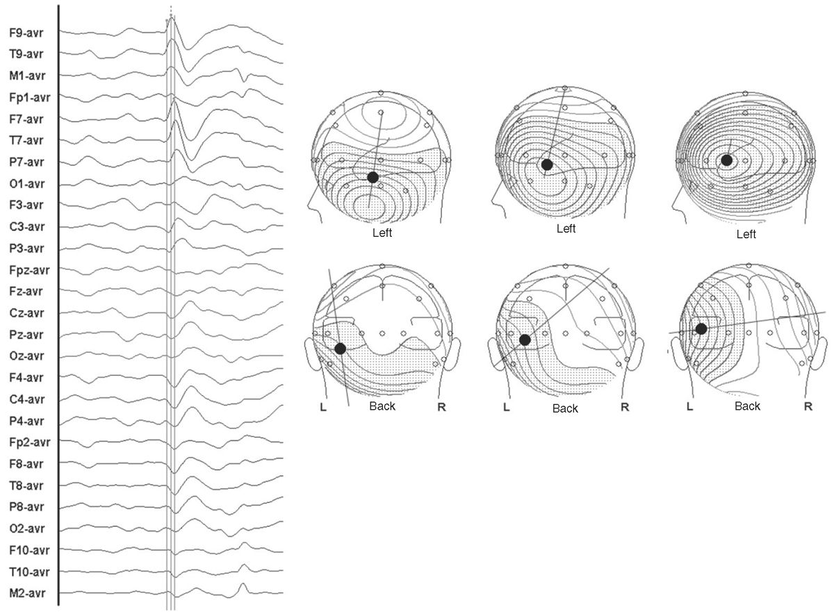
Figure 12.2: Scalp EEG tracing of a left temporal spike is shown at left. Cursors mark three time points on the rising phase to peak of this spike. Topographic maps depict the scalp voltage fields at these three points in isopotential lines (speckled = negative, clear = positive). A 3D line defining field orientation connects the two maxima. Note that early in the spike, the field is vertical and tangential. Later it is oblique, and at the spike peak, the field is horizontal and radial. Such changes in the location of voltage field maxima and field orientation are the result of spike propagation across the cortex. Dipole source modeling predicts that the center of activity of the spike source (identified by a black dot) lies on this 3D line at a location proportionally nearer the maxima of higher amplitude.

If a spike source is spatiotemporally stable, the voltage field will rise and fall in magnitude and reverse in polarity, but the maxima will not move or substantially change in shape. If the spike source is unstable and propagation to the adjacent cortex happens, the geometry of the source will change and the resultant voltage field will also change over time. In this case, the location and shape of maxima will move across the head over the course of the spike, in addition to changes in magnitude and polarity. This change in the spatial distribution of a voltage field over time is the principal marker of propagation (see Fig. 12.2).

Radial fields are typically generated by the crowns of convexity cortex. However, many brain regions that are highly epileptogenic are not found on the cortical convexity. This includes the entire base of the brain, in particular, orbitofrontal and basal temporal regions. These cortices produce EEG fields that are tangential to the head surface rather than radial. Similarly, epileptogenic foci in major fissures, such as Sylvian or interhemispheric, produce tangentially oriented EEG fields. Such sources are important to understand because little or no EEG potential is recorded directly above them, rather the negative and positive EEG fields on the head are displaced on either side of the true source location. In such a situation, considering the negative field maximum as the source origin will result in false localization and even a false lateralization in certain situations (see Fig. 12.1). Simply by inspecting the spike/seizure voltage fields over the head, one can gain considerable information about the likely source of these fields. Such visual analysis is essentially a form of source modeling.

DIPOLE MODELS OF CEREBRAL SOURCES

As noted earlier and in Chapter 2, the cortical sources of EEG spikes or seizure rhythms produce voltage fields on the scalp that are dipolar in nature, possessing a negative and a positive field maximum. The geometry of a cortical source may be complex and comprised of several gyri and sulci; similarly, the cortical voltage fields recorded by subdural electrodes may also be complex. However, above the cortex, including at the scalp, the voltage fields of a convoluted source will add linearly and a simplified dipolar electrical field will predominate. The physical and mathematical explanation for this is found in the multipole expansion. At a distance from the source, more complicated field patterns, such as quadrapoles and octopoles, will diminish, leaving only dipolar patterns. Accordingly, if one is attempting to model cortical sources of EEG, it makes sense to use a model that is dipole-based. It is important to appreciate, however, that a dipole is an unphysiological, biophysical construct—a point-like source with a separation of negative and positive charge that can produce a dipolar field in a conducting volume. The dipole is not the source; it simply is a model of the source.

Dipole localization techniques are based on electric field theory applied to volume conduction, which was developed by Helmholtz (5) in the mid-nineteenth century. Nearly 100 years later, electroencephalographers began to consider the physical relationship between electric fields on the scalp and their underlying sources within the brain (6–9). At the same time, Wilson and Bayley (9) developed a method for calculating the voltage field generated on a spherical volume conductor by a known dipole. In simple terms, if the location, orientation, and strength of a dipolar source within a spherical and homogenous conducting medium are known, one can predict the shape and magnitude of the potential field that is measurable on its surface. The answer to this type of problem has been called the “forward solution,” and it is unique. There is only one field that can be generated by a given dipole. However, the usual clinical problem is the opposite, namely, trying to locate the intracerebral generator having measured the topography of a scalp potential. The answer to this is called the “inverse solution,” and unfortunately, for any given voltage field there is no unique answer. Rather, there are multiple possibilities because the fields of sources in a volume conductor sum linearly (the principle of superposition). Therefore, the field measured by a given electrode array may well be a composite from a number of different sources.

Certain assumptions are necessary to apply dipole modeling to human EEG. First, the brain is often modeled as a sphere of uniform conducting material (10), and concentric shells are added around this to imitate the skull and scalp (11–13). The brain and scalp are usually considered to be of equal resistivity and the intervening skull 20 to 80 times greater. Also, for ease of mathematical modeling, the source of the field is considered to be a point-like dipole. Obviously, the generators of scalp spikes are not point sources, but rather large aggregates of neurons that extend over 10 to 30 cm². However, the combined activity of such a generator region may be modeled effectively by a single dipole. That is to say, the field that would be produced by this “equivalent dipole” is very similar to that of the real source. As a first approximation, the equivalent dipole should reside close to the center of the real generator area and have an orientation that is orthogonal to that of the cortex.

Single-Moving Dipole Model

The most common form of source localization is the instantaneous, single-dipole inverse solution. This procedure takes the voltage values from all electrodes at a given instant in time and searches for an equivalent dipole within a spherical head that could generate such a field. Various algorithms exist for identifying an equivalent dipole source (14–16). Most of these algorithms use an iterative minimizing approach, whereby an estimate of source location is made; the forward solution is performed, and the difference between the forward solution and the actual measured field is characterized. Subsequent random movements of the dipole model attempt to minimize this difference. When the smallest difference is obtained, the putative dipolar source has been identified. This method defines a single equivalent source for a voltage field at one point in time. Regardless of the complexity of the real cerebral sources, the resultant compound activity is simplified into that of a single-dipole generator.

Spike voltage fields evolve over time, but the instantaneous single-dipole technique models the field at only one instant. Temporal evolution of a voltage field can, however, be described by a series of sequential single dipoles that can move in position and orientation over time, if the field changes. These can be displayed in one image as a “moving” dipole (17,18). For some spikes, repeated dipole solutions are very consistent during the course of the potential, varying only in magnitude and little in position or orientation (Fig. 12.3). A single-dipole model fits these types of data well and suggests a discrete cerebral generator or nearly synchronous activation of several generator regions. For other spikes, sequential solutions over the potential’s time course show progressive drift in dipole location and rotation of vector orientation (Fig. 12.4). Such behavior of the dipole model is incompatible with a single-generator region and suggests asynchronous activation of different cortical areas.

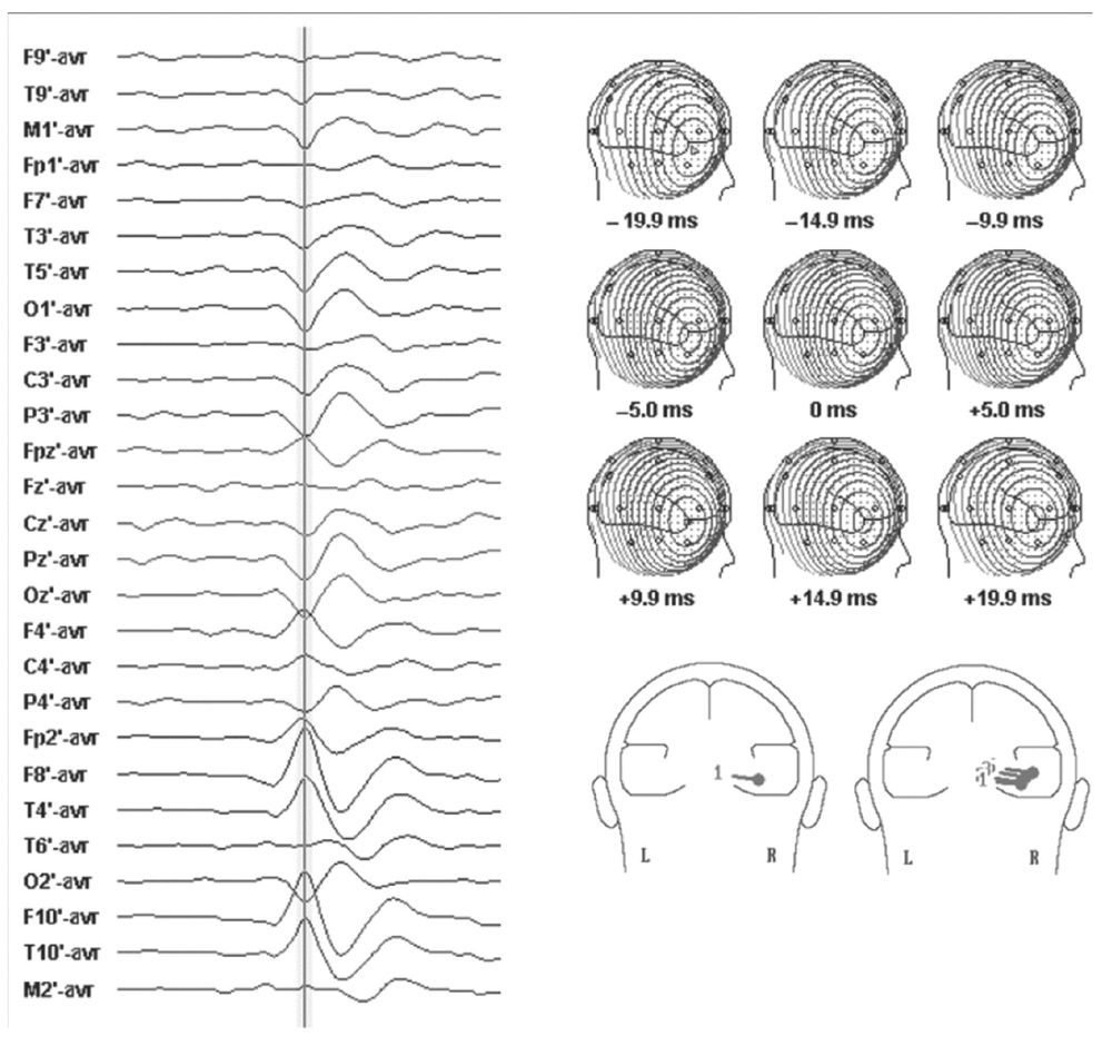
Figure 12.3: Left: Scalp EEG of a right temporal spike with a horizontal, radial field orientation. Cursor denotes 0 millisecond latency. Top right: Sequential voltage topography of the spike. Note stable shape of the fields over 40 milliseconds. Bottom right: Single and moving dipole models of the spike. Note that voltage field stability and tight cluster of the moving dipole model suggest a simple source for which a single-dipole model is appropriate.

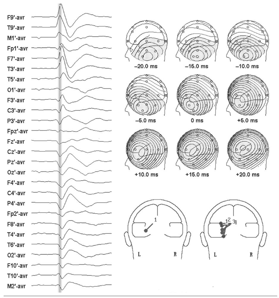
Figure 12.4: Left: Scalp EEG of a left temporal spike with an elevated, combined radial/tangential field orientation. Cursor denotes 0 millisecond latency. Top right: Progressive change in the sequential voltage topography of the spike is evident. Bottom right: Single and moving dipole models of the spike. Single dipole at spike peak is oblique in orientation, while moving dipole model shows a progression in dipoles from vertical tangential to horizontal radial, suggesting propagation from base to lateral temporal cortex.

The direction of dipole movement can convey useful information about the likely path of spike propagation, as long as it is simple and unidirectional. Moving dipoles that spiral in a loop or make sudden turns in direction or position are usually the result of fields created by superposition of early source repolarization and later source depolarization or several different asynchronous sources. Therefore, one-dipole solutions can be misleading, particularly at later latencies when propagation is likely to have occurred, resulting in increased source complexity. Several investigators have concluded that modeling the rising phase of the spike is more likely to represent the initial spike source (2,3,19,20). Obviously, there is a trade-off because the earlier time points typically have lesser signal-to-noise (S/N), which may make modeling less accurate. Averaging closely similar spikes or sequential ictal waveforms can improve the S/N, which will provide a more confident solution (21).

Spatiotemporal Multiple-Dipole Model

Although the moving single-dipole model will characterize simple propagation, it is overly simplistic to think that small brain regions are activated briefly in sequence. It is more reasonable that adjacent cortical areas are activated for a longer period, but not synchronously. Source modeling with single instantaneous dipoles cannot take into consideration such an overlap of activity of multiple generators, nor can it decompose the voltage fields produced by this superposition. Spatiotemporal source modeling is, however, an approach based on this rationale (22–24). Dipoles are fixed in location and orientation but can vary over time in strength and polarity to explain the temporal evolution of a voltage field. Sufficient degrees of freedom are obtained to calculate multiple dipoles from this positional constraint and from modeling over several time points. The solution for a given data set reveals not only a best-fit location for the model, but also the putative activity of each dipole over time in the form of a source potential (Fig. 12.5).

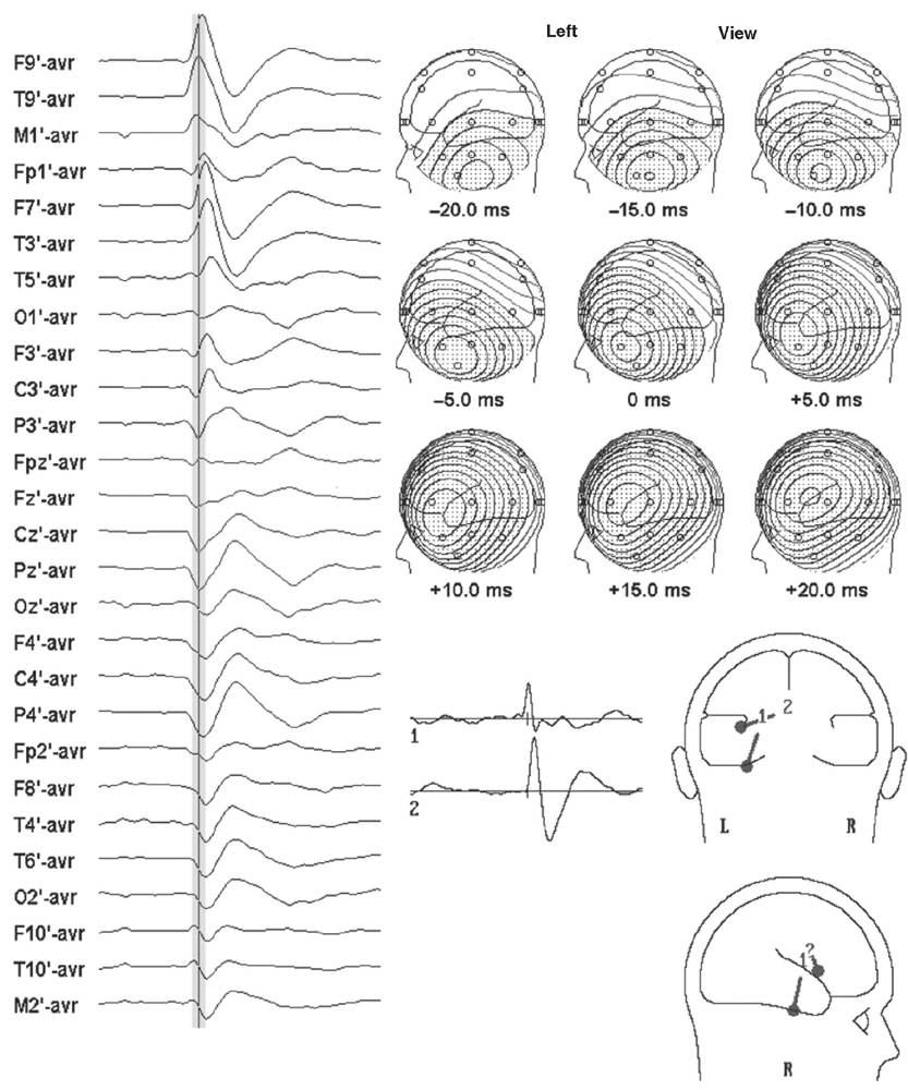
Figure 12.5: Same EEG and sequential voltage topography as depicted in Fig. 12.4. Bottom right: A spatiotemporal dipole model with two dipoles, (1) vertical tangential and (2) horizontal radial, can explain the voltage field evolution over the time course of the spike, if dipole 1 has the source activity of trace 1 and dipole 2 has the source activity of trace 2. The spatiotemporal dipole model also suggests spike propagation from base to lateral temporal lobe.

Because there is no unique solution when trying to identify several sources that may underlie a voltage field that is a composite, it is necessary to use modeling strategies to constrain the solutions to those that are most realistic. Two major categories of strategies include those based on sequential temporal activation of adjacent generator areas and those based on the orientation of the cortical areas likely to be involved in the process. Implicit in the “temporal” strategy is the idea that the earliest part of a spike waveform is more likely to be the product of a single source than are later segments. Accordingly, one should first attempt to model the early part of the field evolution as a single dipole, rather than the spike peak, for example. Additional dipoles are used in sequence to model the residual field left unexplained by the preceding dipole(s). If the initial equivalent source explains, in spatiotemporal terms, the entire spike field evolution, the generator is rather discrete or simple in character. Commonly, however, two or sometimes three dipoles are necessary to explain the time course of even “focal” spike data. The spatiotemporal technique attempts to find the fewest number of fixed equivalent sources that can explain field evolution by a temporal overlap of activity among them.

Modeling strategies using anatomic constraints can also be useful. The mathematics of unconstrained inverse solutions considers any position within the spherical head model and any orientation of dipole vector to be equally likely as a source. This is obviously not true biologically. Spikes arise from the cortex that has limited and definable locations and orientations. Of the two, it is more useful to specify the orientation of possible equivalent sources. As noted previously, it is reasonable to consider for purposes of modeling, only the orientations of major lobar surfaces. For the temporal lobes, these orientations are horizontal radial for the lateral convexity cortex, vertical tangential for the basal cortex and superior temporal plane, and AP horizontal tangential for the temporal tip. One approach in using this strategy for the temporal lobes is to create a priori a multiple spatiotemporal dipole model of major lobar surfaces, based on specific orientations obtained from brain imaging studies, and to note from the source potentials to what extent each dipole can contribute to explaining spike voltage fields over time (25–28).

INTERPRETATION OF DIPOLE MODELS

The clinical interpretation of dipole source models requires an appreciation for the weaknesses in the modeling assumptions and the complexity of source geometry and physiology. It is clear from studies of simultaneous scalp and intracranial EEG that the sources of scalp spikes and seizure rhythms are quite large, namely 10 to 30 cm². A point source dipole is a simple model of this extended cortical generator, and in order for it to be useful, it must be interpreted properly. As noted previously, EEG dipoles model major cortical surfaces, not individual gyri or sulci.

Dipole location identifies only the “center of activity” of the cortical source and certainly not its extent. Because this point source model tries to explain the scalp field resulting from an extended source, the model dipole is typically located deep to actual source cortex. Dipole localization techniques are least accurate in depth determinations because this estimation depends on the size of the generator region. Single-dipole solutions provide a reasonable approximation for superficial cortical sources, if their diameter is smaller than 2 cm, such as with somatosensory-evoked potentials (23). Activation of a larger area of cortex, as is the case of epileptiform spikes, produces a more diffuse scalp field that would have to be modeled as a deeper equivalent dipole. Think of a flashlight producing an illuminated spot on a wall. In order for the flashlight to produce a larger spot, equivalent to a larger field, it must be farther from the wall, or in the case of a dipole, deeper in the brain. Accordingly, one should not be concerned about dipole models that localize to white matter.

It is the dipole orientation that identifies the likely source cortex within the region (17,18,29). Dipole orientation conveys the net orientation of the pyramidal cells generating the field and this is orthogonal to the net orientation of the generator cortex. A simple step in EEG dipole interpretation is to project the dipole vector out to the cortical surface. If the EEG field is principally radial, this projection should intersect source cortex that has a net orientation that is orthogonal to the dipole vector (Fig. 12.6). If there is no cortex in the region of a dipole model that has an appropriate orientation, the validity of the source solution should be questioned.

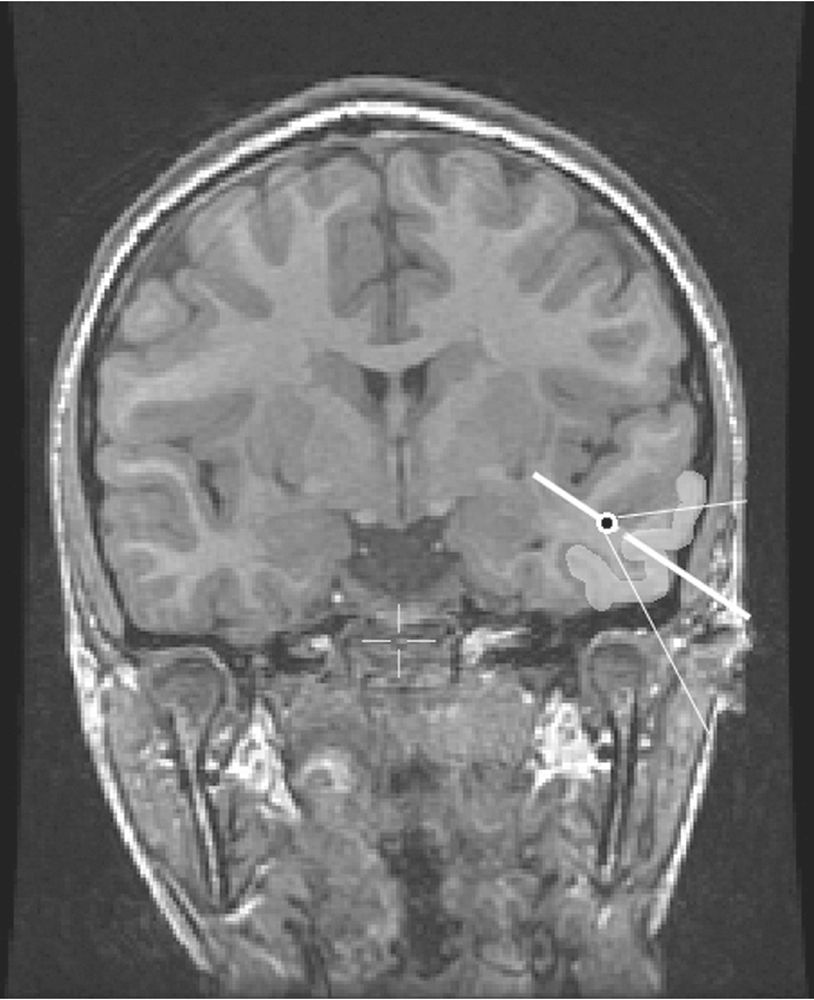
Figure 12.6: In order to simulate the broad scalp voltage field generated by a large cortical source (lightened left temporal cortex), an equivalent dipole (black dot)

Stay updated, free articles. Join our Telegram channel

Join