Doppler Echocardiography and Color Flow Imaging: Comprehensive Noninvasive Hemodynamic Assessment
Hemodynamic assessment is a major part of a routine echocardiography examination. Stroke volume, cardiac output, intracardiac pressures, pressure gradients, and vascular resistance are reliably determined with two-dimensional (2D), Doppler, and color flow imaging echocardiography. This noninvasive measurement of hemodynamic variables not only has replaced many invasive hemodynamic procedures but it also can be superior to them under certain circumstances. Because many therapeutic decisions, including surgical intervention, are based on echocardiography, it is critical that everyone involved in the care of cardiac patients as well as everyone involved in performing echocardiography understand how a hemodynamic assessment is performed by echocardiography and know its advantages and potential limitations.
Doppler Echocardiography
Doppler in the heart and great vessels and is based on the Doppler effect, which was described by the Austrian physicist Christian Doppler in 1842 (1). The Doppler effect is the increase in sound frequency as a sound source moves toward the observer and the decrease in sound frequency as the source moves away from the observer. In the circulatory system, the moving target is the red blood cell. When an ultrasound beam with known frequency (fo) is transmitted to the heart or great vessels, it is reflected by the red blood cells. The frequency of the reflected ultrasound waves (fr) increases when the red blood cells are moving toward the source of ultrasound. Conversely, the frequency of reflected ultrasound waves decreases when the red blood cells are moving away from the source. The change in frequency between the transmitted sound and the reflected sound is termed the frequency shift (Δ f) or Doppler shift (fr-fo). The Doppler shift depends on the transmitted frequency (fo), the velocity of the moving target (v), and the angle (θ) between the ultrasound beam and the direction of the moving target as expressed in the Doppler equation (Fig. 4-1):
where c is the speed of sound in blood (1,540 m/s). If the angle θ is 0 degree (i.e., the ultrasound beam is parallel with the direction of blood flow), the maximal frequency shift is measured because the cosine of 0 degree is 1. Note that as angle θ increases, the corresponding cosine becomes progressively less than 1, and this will result in underestimation of the Doppler shift (Δf) and, hence, peak velocity, because peak flow velocity is derived from Δf by rearranging the Doppler equation:
Blood flow velocities determined by Doppler echocardiography are used, in turn, to derive various hemodynamic data (see below).
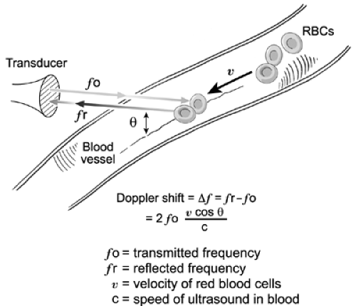 Figure 4-1 Diagram of the Doppler effect (see text for explanation). RBCs, red blood cells. |
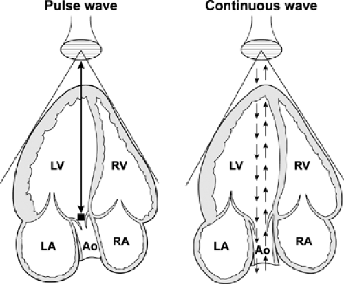 Figure 4-2 Drawing of pulsed wave and continuous wave Doppler echocardiography from the apical view (see text for explanation). Ao, aorta; LA, left atrium; LV, left ventricle; RA, right atrium; RV, right ventricle. |
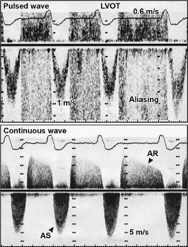 Figure 4-3 Representative pulsed wave and continuous wave Doppler spectra from a 60-year-old patient who has aortic stenosis (AS) and aortic regurgitation (AR). The pulsed wave Doppler sample volume is placed at the left ventricular outflow tract (LVOT), and the Doppler spectrum shows systolic LVOT velocity and turbulent diastolic signal of aortic regurgitation recorded on both sides of the baseline. Although AR flow is toward the transducer, aliasing (velocity wraparound) occurs because of high velocity (4–5 m/s). Continuous wave Doppler detects flow velocities all along its beam (LVOT and aortic valve) and is able to record high velocity. Systolic flow away from the transducer (spectrum below the baseline) represents flow across the stenotic aortic valve (AS) and diastolic flow is from AR. Peak AS velocity across the stenotic valve varies (5.0–5.5 m/s) because of atrial fibrillation. |
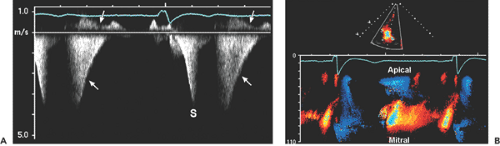 Figure 4-4 A: Continuous wave Doppler recording from the apex. There is an unusual velocity recording (upward arrows) away from the apex with a velocity close to 4 m/s, which occurs about 100 ms before mitral inflow (downward arrows). S indicates systolic flow velocity away from the apex; it has a dagger configuration. B: Color M-mode from the same patient shows that the unusual flow comes from the apical area (blue) to the mid-cavity, starting before mitral inflow, typical of mid-cavitary obstruction. During isovolumic relaxation period, there is a dyssynchrony of myocardial relaxation that results in a pressure gradient from the apex to the basal segment across the obstructed mid-cavity. |
The most common uses of Doppler echocardiography are the pulsed wave and continuous wave forms (Fig. 4-2). Both modalities are essential parts of a Doppler echocardiography examination and provide complementary information. In the pulsed wave mode, a single ultrasound crystal sends and receives sound beams. The crystal emits a short burst of ultrasound at a certain frequency (pulse repetition frequency). The ultrasound is reflected from moving red blood cells and is received by the same crystal. Therefore, the maximal frequency shift that can be determined by pulsed wave Doppler is one-half the pulse repetition frequency; this is called the Nyquist frequency. If the frequency shift is higher than the Nyquist frequency, aliasing occurs; that is, the Doppler spectrum is cut off at the Nyquist frequency, and the remaining frequency shift is recorded on the top or bottom of the opposite side of baseline (Fig. 4-3).
Pulsed wave Doppler measures flow velocities at a specific location within a “sample volume.” The pulse repetition frequency varies inversely with the depth of the sample volume: the shallower the location of the sample volume, the higher the pulse repetition frequency and Nyquist frequency. In other words, higher velocities can be recorded without aliasing by pulsed wave Doppler the closer the sample volume is to the transducer.
Pulsed wave Doppler measures flow velocities at a specific location within a “sample volume.” The pulse repetition frequency varies inversely with the depth of the sample volume: the shallower the location of the sample volume, the higher the pulse repetition frequency and Nyquist frequency. In other words, higher velocities can be recorded without aliasing by pulsed wave Doppler the closer the sample volume is to the transducer.
In the continuous wave mode, the transducer has two crystals: one to send and the other to receive the reflected ultrasound waves continuously. Therefore, the maximal frequency shift that can be recorded by continuous wave Doppler is not limited by the pulse repetition frequency or Nyquist phenomenon. Unlike pulsed wave Doppler, continuous wave Doppler measures all the frequency shifts (i.e., velocities) present along its beam path; hence, it is used to detect and to record the highest flow velocity available. Occasionally, recording of a high-velocity flow is the first clue to an unsuspected lesion within the path of a continuous wave Doppler beam (Fig. 4-4). Continuous wave Doppler usually is performed with either an image-guided or nonimaging transducer. A small nonimaging transducer (pencil probe) is more suitable for interrogation of a high-velocity jet from multiple windows, including areas between the ribs. An image-guided continuous wave examination is more helpful when the direction of blood flow is eccentric or the amount of desired blood flow is trivial. The characteristics and clinical applications of these Doppler modalities are summarized in Table 4-1. Table 4-2 lists the mean and range of maximal velocities recorded from normal subjects by Doppler echocardiography. Echocardiographers should be familiar with the characteristic configuration and timing of normal and abnormal Doppler signals (Figs. 4-4 and 4-5).
Color Flow Imaging
Color flow imaging, based on pulsed wave Doppler principles, displays intracavitary blood flow in three colors (red, blue, and green) or their combinations, depending on the velocity, direction, and extent of turbulence (2). It uses multiple sampling sites along multiple ultrasound beams (multigated). At each sampling site (or gate), the frequency shift is measured, converted to a digital format, automatically correlated (autocorrelation) with a preset color scheme, and displayed as color flow superimposed on 2D imaging (Fig. 4-6A). Blood flow directed toward the transducer has a positive frequency shift (i.e., reflected ultrasound frequency is higher than the transmitted frequency) and is color-coded in shades of red. Blood flow directed away from the transducer has a negative frequency shift and is color-coded in shades of blue. Each color has multiple shades, and the lighter shades within each primary color are assigned to higher velocities within the Nyquist limit. When flow velocity is higher than the Nyquist frequency limit, color aliasing occurs and is depicted as a color reversal (Fig. 4-6B). With each multiple of the Nyquist limit, the color repeatedly reverts to the opposite color. Turbulence (i.e., blood moving in multiple directions with multiple velocities) is characterized by the presence of variance. The degree of the variance from the mean velocity can be coded as a variance color, usually a shade of green. Therefore, abnormal blood flow is easily recognized by combinations of multiple colors according to the direction, velocity, and degree of turbulence (Fig. 4-6). The width and size of abnormal intracavitary flows are
used to semiquantify the degree of valvular regurgitation or cardiac shunt.
used to semiquantify the degree of valvular regurgitation or cardiac shunt.
Table 4-1 Comparison of pulsed wave and continuous wave Doppler | |||||||||||||
|---|---|---|---|---|---|---|---|---|---|---|---|---|---|
|
Because the types and shades of color flow imaging are determined by the direction and velocity of blood flow, color flow imaging is an excellent way to visualize simultaneously all the intracavitary blood flow within a color flow sector. The size and location of a color flow imaging sector are easily adjusted by a trackball. Color flow imaging is also an essential part of hemodynamic assessment. An important example is the calculation of flow rate at proximal isovelocity surface area (PISA) to determine mitral or aortic regurgitant volume and regurgitant orifice area (3). Color flow imaging also is used in color M-mode of the mitral inflow to determine diastolic function and the rate of flow propagation as well as the timing of intracardiac blood flow (Figs. 4-4 and 4-7).
Table 4-2 Normal maximal velocities (m/s): Doppler measurements | ||||||||||||||||||||||||||||||||||||||||
|---|---|---|---|---|---|---|---|---|---|---|---|---|---|---|---|---|---|---|---|---|---|---|---|---|---|---|---|---|---|---|---|---|---|---|---|---|---|---|---|---|
| ||||||||||||||||||||||||||||||||||||||||
Comprehensive hemodynamic data can be obtained with 2D, Doppler, and color flow imaging. To use this powerful hemodynamic technique to the fullest potential, echocardiographers need to understand and memorize several essential hemodynamic principles. It needs to be emphasized that no invasive or noninvasive hemodynamic measurements are perfect, and many factors influence cardiac hemodynamic calculations. Mastery of the following concepts will minimize calculation errors and help echocardiographers avoid pitfalls in noninvasive hemodynamic calculations. All hemodynamic data, whether obtained invasively or noninvasively, should be
interpreted in the context of and correlated with the clinical presentation.
interpreted in the context of and correlated with the clinical presentation.
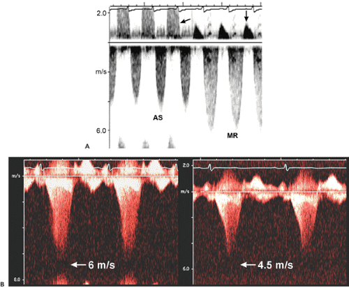 Figure 4-5 A: Continuous wave Doppler records all velocities along its ultrasound beam path. Therefore, a slight angulation of the transducer may record entirely different velocities. This continuous wave recording was obtained from the apical window with a pencil probe in a patient who had severe aortic stenosis (AS) and moderate mitral regurgitation (MR). A slight change in the direction of the continuous wave Doppler probe recorded both AS and MR signals as well as aortic regurgitation (left arrow) and mitral inflow (down arrow) during diastole. Note that the duration and peak velocity of AS are shorter and lower, respectively, than those of MR. B: Typical continuous wave Doppler recordings from a patient with obstructive hypertrophic cardiomyopathy. Both recordings have the shape of a “dagger.” However, the signal on the left comes from mitral regurgitation and the signal on the right from an obstructed left ventricular outflow tract. (See Chapter 15 for more detail.) |
Transvalvular Gradients
Based on the Doppler shift, Doppler echocardiography measures blood flow velocities in the cardiac chambers and great vessels. Blood flow velocities can be converted to pressure gradients (in millimeters of mercury [mm Hg]) according to the Bernoulli equation (Fig. 4-8).
In most clinical situations, flow acceleration and viscous friction terms can be ignored. Furthermore, flow velocity proximal to a fixed orifice (v1) is much lower than the peak flow velocity (v2); hence, v1 also can frequently be ignored. Therefore, pressure gradient (or pressure drop) across a fixed orifice can be calculated with the simplified Bernoulli equation:
Pressure gradient (Δ P) = 4 × (v2)2 or (2 v2)2
Blood flow velocity measured with Doppler echocardiography is an instantaneous event, and the pressure
gradients derived from Doppler velocities are instantaneous gradients. When maximal Doppler velocity is converted to pressure gradient using the simplified Bernoulli equation, it represents the maximal instantaneous gradient. It should be noted that the maximal instantaneous gradient obtained with Doppler echocardiography is always higher than the peak-to-peak gradient measured in the catheterization laboratory (Fig. 4-9). Peak-to-peak gradient in aortic stenosis is the pressure difference between the peak left ventricular (LV) and peak aortic pressures, which do not occur simultaneously and, hence, is a nonphysiologic measurement. Mean gradient is an average of pressure gradients during the entire flow period, and the mean gradient obtained with Doppler echocardiography has been shown to correlate well with one measured simultaneously by cardiac catheterization. From the Doppler tracing, the mean gradient can be obtained by tracing the velocity signal and using the built-in calculation package (Fig. 4-10). Several studies have validated that Doppler-derived pressure gradients are highly accurate and have an excellent correlation with catheter-derived pressure gradients across a left ventricular outflow tract (LVOT) or right ventricular outflow tract (RVOT) obstruction, mitral stenosis, pulmonary artery band, and various prosthetic valves (4,5,6,7,8,9) (Fig. 4-11). In some clinical situations, the Doppler-derived pressure
gradient is more reliable than a catheter-derived gradient. Transmitral (normal, stenotic, native, or prosthetic valve) pressure gradient may be overestimated by cardiac catheterization if pulmonary capillary wedge pressure (PCWP) is used (instead of direct left atrial [LA] pressure) to calculate the pressure gradient (10).
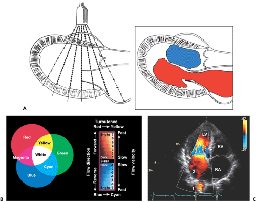 Figure 4-6 A: Drawing illustrating how color flow imaging is performed and displayed. The dots indicate multiple sampling sites (gates). The frequency shift measured at each gate is correlated automatically (autocorrelation) and converted to a preset color scheme (red for flow toward and blue for flow away from the transducer). B: Color flow imaging is displayed using the three colors red, blue, and green and their combinations based on the velocity, direction, and turbulence of flow. C: Color flow imaging from the apical four-chamber view of the left ventricle (LV), mitral valve, and left atrium. Color flow imaging of the pulmonary vein (1), left atrium (2), and mitral valve (3) indicates that blood flow is toward the apex during diastole, and flow velocity is highest at the mitral valve (3), followed by that of the pulmonary vein (1), and left atrium (2). The color of blood flow changes from dark orange in the left atrium, to light yellow, to blue (with aliasing), then again to light yellow, and orange. RA, right atrium; RV, right ventricle. (B From Omoto and Kasai [2]. Used with permission.) |
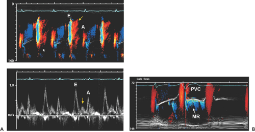 Figure 4-7 A: Color M-mode of mitral inflow (top), indicating the timing and velocity of diastolic velocities, E and A. Arrow (top) indicates a mid-diastolic flow, confirmed by pulsed wave Doppler echocardiography (arrow, bottom). B: Color M-mode from the mitral valve demonstrating an increased amount of mitral regurgitation (MR) after a premature ventricular contraction (PVC). |
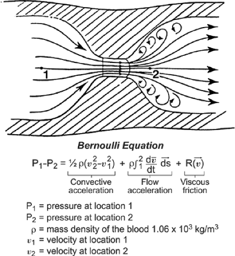 Figure 4-8 Diagram of blood flow through a narrowed orifice to illustrate the Bernoulli equation, which measures the pressure gradient across the orifice using blood flow velocities. The Bernoulli equation has three components: convective acceleration, flow acceleration, and viscous friction. Because the velocity profile in the center of the lumen is usually flat, the viscous friction factor can be ignored in the clinical setting. The flow acceleration term causes a delay between the pressure drop curve and the velocity curve but provides a reasonably accurate estimation of pressure gradient, and this flow acceleration factor is ignored. Therefore, in a clinical setting, the flow gradient across a narrowed orifice can be derived from the convective acceleration term alone. (From Hatle and Angelsen [1]. Used with permission.) |
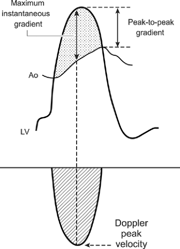 Figure 4-9 Diagram of pressure tracings of left ventricle (LV) and aorta (Ao) in aortic stenosis along with the corresponding Doppler velocity spectrum. It is important to understand how different pressure gradients are derived. The average of pressure differences between LV and Ao (stippled area) represents the mean gradient (see text). |
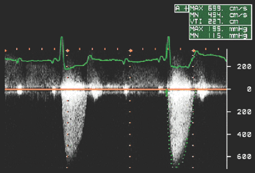 Figure 4-10 Continuous wave Doppler signal of the aortic valve from the apex in an 87-year-old woman with severe aortic stenosis. Peak velocity is 7.0 m/s, and the tracing of the velocity yields a mean gradient (MN) of 115 mm Hg. A built-in calculation package also provides peak instantaneous gradient (MAX), and time velocity integral (VTI). |
Intracardiac Pressures
The velocity across an orifice in the cardiovascular system is related directly to the pressure difference (or drop) between the proximal and distal portions of the orifice, according to the Bernoulli equation. Therefore, flow velocities recorded by Doppler echocardiography are used to determine various intracardiac pressures, as shown in Table 4-3.
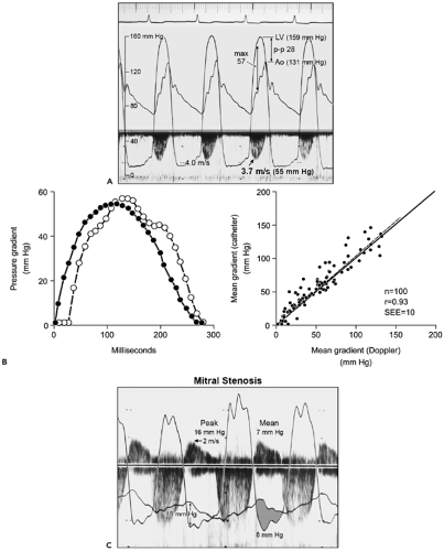 Figure 4-11 A: Simultaneous Doppler and cardiac pressure recordings show an excellent correlation between Doppler-derived and catheter-derived pressure gradients in aortic stenosis. Peak Doppler velocity (3.7 m/s) from the third cardiac cycle is converted to a maximal instantaneous gradient (max) of 55 mm Hg, which corresponds well to the maximal gradient determined by catheter (57 mm Hg) but not to the peak-to-peak (p–p) gradient of 28 mm Hg. LV, left ventricle; Ao, aorta. (B from
Get Clinical Tree app for offline access
Currie PJ, Seward JB, Reeder GS, et al. Continuous wave Doppler echocardiographic assessment of severity of calcific aortic stenosis: A simultaneous Doppler-catheter correlative study in 100 adult patients. Circulation, 1985;71:1162–1169 . Used with permission.). B: Digitization of the Doppler spectral velocity envelope and (LV-Ao) pressure waveforms of the third beat in A. Left, The phase delay of the catheter gradient (closed circles) compared with the Doppler-derived gradient (open circles) is related to the fluid-filled catheter system. Right, Plot of mean gradients by Doppler echocardiography and catheterization shows a good correlation in 100 patients with aortic stenosis. r, correlation coefficient; SEE, standard error of estimate. C:
Stay updated, free articles. Join our Telegram channel
Full access? Get Clinical Tree


|