, is simply a point estimate for the population mean. This will be further discussed in the following section. The median is the middle measurement when all of the measurements are sorted in ascending or descending order, which can be a better measure of central tendency in skewed distributions. In normal (bell-shaped) distributions, the average and median values are the same. The mode is the measurement with the highest frequency. Based on these three measures of central tendency, one can understand the shape of the distribution. Furthermore, depending on the type of measurements and shape of the distribution, one may choose one or more of these measures of central tendency to describe their data set.
25.2.2 Measures of Spread: Range, Variance, and Standard Deviation
Sample range is the difference between the highest and the lowest measurements. Therefore, it is a very sensitive measure of variability because it is influenced by the extreme observations. For situations in which there are extreme observations, some researchers use the interquartile range (IQR) which represents the difference between the 25th percentile and 75th percentile. Sample variance (s 2) is another important measure of variability, which is calculated by the following formula (Eq. 25.1), where x i are the individual measurements,  is the sample mean and n is the sample size:
is the sample mean and n is the sample size:(25.1)
Since the unit of variance is squared of the original unit of measure, the sample standard deviation (s) is often used as another measure of spread, which is simply the square root of the sample variance (Eq. 25.2):
(25.2)
It is important to distinguish the difference between population and sample measures of spread. For example, population standard deviation (σ) is a measure of spread over the entire population of size N with a mean of μ (Eq. 25.3); similarly, population variance is denoted by σ 2. The reason for using “n − 1” in calculating sample variance (s 2) and standard deviation (s) is to ensure that the estimates for variability remain unbiased. This concept is discussed in standard statistical textbooks, and we refer the reader to Fundamentals of Biostatistics by Bernard Rosner for additional information.
(25.3)
25.2.3 Normal Distributions
In practice, many measurements including weight and height have a bell-shaped distribution. Mathematically these distributions can be characterized by a normal (Gaussian) distribution with mean μ and standard deviation σ. The normal distribution is symmetrical and has the property that about 68 % of the observations lie within one standard deviation from the mean, 95 % within 2 standard deviations, and 99.7 % within 3 standard deviations (Fig. 25.1).
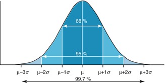
Fig. 25.1
A normal distribution of the population with mean μ and standard deviation (sigma)
25.2.4 Skewed Distributions
Not all distributions are normal in nature. In fact, skewed distributions are common in clinical data. In a negatively skewed distribution (i.e., skewed towards the left), the mean is less than the median. In a positively skewed distribution (i.e., skewed towards the right), the median is less than the mean. In a bimodal distribution, there are two modes, one mean, and one median. For irregular distributions, one may be interested in describing the data in terms of the median and interquartile range (Fig. 25.2).
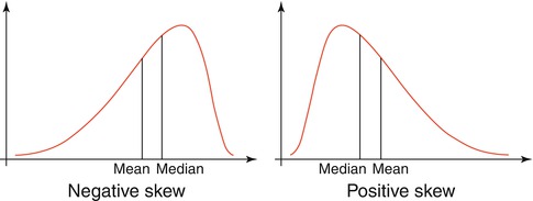
Fig. 25.2
A negatively skewed curve has a mode that is greater than the median, which is greater than the mean (left-skewed). A positively skewed curve has the opposite finding (right-skewed)
25.2.5 Estimation and Bias
As stated earlier, one of the objectives of statistics is to infer the properties of the underlying population from a sample (i.e., subset of the population). Statistical inference can be subdivided into two main areas: estimation and hypothesis testing. Estimation is concerned with estimating the values of specific population parameters. It is therefore, very important to understand the relationships between the sample characteristics and population parameters [5–10].
25.2.6 Point and Interval Estimators for the Population Mean
A natural estimator for μ is the sample mean  , which is referred to as a point estimate. Suppose we want to determine the appropriate sample size for estimating the mean of a population (μ) which is unknown. We can start by taking a random sample to determine the sample mean and sample variance. However, the sample mean values can change from sample to sample. Therefore, it is necessary for us to determine the variation in the point estimate (e.g., sample mean). Assuming that the sample size is large (n > 30), we can determine an interval estimate (e.g., 95 % confidence interval) for the population parameters. For example, if the population parameter is μ, a 95 % confidence interval can be calculated by the following formula (Eq. 25.4). The value 1.96 is the exact value determined from the normal distribution, which is based on the fact that 95 % of the measurements are within 1.96 (approximately 2) standard deviations of the mean.

, which is referred to as a point estimate. Suppose we want to determine the appropriate sample size for estimating the mean of a population (μ) which is unknown. We can start by taking a random sample to determine the sample mean and sample variance. However, the sample mean values can change from sample to sample. Therefore, it is necessary for us to determine the variation in the point estimate (e.g., sample mean). Assuming that the sample size is large (n > 30), we can determine an interval estimate (e.g., 95 % confidence interval) for the population parameters. For example, if the population parameter is μ, a 95 % confidence interval can be calculated by the following formula (Eq. 25.4). The value 1.96 is the exact value determined from the normal distribution, which is based on the fact that 95 % of the measurements are within 1.96 (approximately 2) standard deviations of the mean.(25.4)
The quantity to the right of the mean in Eq. 25.4 is known as the margin of error or the bound on the error of estimation (B). In general, as sample size increases, B decreases. However, this inverse relationship is not linear. In order to decrease B by half, one must increase the sample size by a factor of 4. This relationship between margin of error, B, and sample size allows researchers to calculate the appropriate sample size to achieve the desired bound on the error with 95 % confidence and will be further elaborated in the sample size determination section.
25.2.7 Standard Error of the Mean
The standard error of the mean (SEM) or standard error (SE) is the standard deviation of sample mean. There is a mathematical relationship between the standard deviation of the measurements in the population and the SEM. This mathematical relationship helps to calculated SEM based on one random sample of size n. SEM is equal to the standard deviation divided by the square root of the sample size n. The SEM is affected by the sample size; as the sample size increases, the SEM decreases (Eq. 25.5):

(25.5)
25.2.8 Point and Interval Estimators for the Population Proportion
In clinical studies, one is often interested in assessing the prevalence of a certain characteristic of the population. In this case, it is important to determine the point and interval estimators for the population proportion (p). The point estimator for the population proportion  is defined as the proportion of the observed characteristic of interest in the sample (Eq. 25.6):

is defined as the proportion of the observed characteristic of interest in the sample (Eq. 25.6):(25.6)
For large samples with a 95 % confidence interval, the population proportion p is calculated as follows:
(25.7)
The quantity to the right of the sample proportion in Eq. 25.7 is known as the margin of error or the bound on the error of estimation (B). As shown before in the case of point estimates for the population mean, this relationship can be used to estimate the appropriate sample size, which will be explained later.
25.2.9 Bias
Generally, bias is defined as “a partiality that prevents objective consideration of an issue.” In statistics, bias means “a tendency of an estimate to deviate in one direction from a true value.” In terms of the population means and proportion estimates described in the previous sections, bias can be defined as:
(25.8)
From a statistical perspective, an estimator is considered unbiased if the average bias based on repeated sampling is zero. For example, is an unbiased estimator of μ and
  is an unbiased estimator for p. However, there are multiple sources of bias inherent in any study that may occur during the course of the study, from allocation of participants and delivery of interventions to measurement of outcomes. Bias can also occur before the study begins or after the study during analysis. Late-look bias occurs with re-examination and re-interpretation of the collected data after the study has been unblinded. Lead-time bias occurs when earlier examination of patients with a particular disease leads to earlier diagnosis, giving the false impression that the patient will live longer. Measurement bias occurs when an investigator familiar with the study does the measurement and makes a series of errors towards the conclusion they expect. Recall bias occurs when patients informed about their disease are more likely to recall risk factors than uninformed patients. Sampling bias occurs when the sample used in the study is not representative of the population and so conclusions may not be generalizable to the whole population. Finally, selection bias occurs when the lack of randomization leads to patients choosing their experimental group which could introduce confounding [11–14].
is an unbiased estimator of μ and is an unbiased estimator for p. However, there are multiple sources of bias inherent in any study that may occur during the course of the study, from allocation of participants and delivery of interventions to measurement of outcomes. Bias can also occur before the study begins or after the study during analysis. Late-look bias occurs with re-examination and re-interpretation of the collected data after the study has been unblinded. Lead-time bias occurs when earlier examination of patients with a particular disease leads to earlier diagnosis, giving the false impression that the patient will live longer. Measurement bias occurs when an investigator familiar with the study does the measurement and makes a series of errors towards the conclusion they expect. Recall bias occurs when patients informed about their disease are more likely to recall risk factors than uninformed patients. Sampling bias occurs when the sample used in the study is not representative of the population and so conclusions may not be generalizable to the whole population. Finally, selection bias occurs when the lack of randomization leads to patients choosing their experimental group which could introduce confounding [11–14].25.3 Hypothesis Testing
25.3.1 Developing a Hypothesis
A research question can be formulated into null and alternative hypotheses for statistical testing. The null hypothesis states that there is no difference between the parameter of interest and the hypothesized value of the parameter. Whereas the alternative hypothesis is that there is some kind of difference. The alternative hypothesis cannot be tested directly; it is accepted by default if the test of statistical significance rejects the null hypothesis. In the case of comparing two population parameters, the null hypothesis is that there is no difference between groups (A or B) on the measured outcome, whereas the alternative hypothesis is that there is a difference between the measured outcome and the group (A or B). Alternatively, the null hypothesis can be written as no association between group (A or B) and measured outcome vs. alternative hypothesis that there is an association between group (A or B) and the measured outcome. In later sections, you will see that some researchers prefer to write the hypotheses in terms of the ratio of the two population parameters [e.g., relative risk (RR) or odds ratio (OR)]. In this case the null hypothesis can be written as RR = 1 (OR = 1) vs. RR ≠ 1 (OR ≠ 1).
25.3.2 Other Elements of Testing Hypothesis
In addition to the null and alternative hypotheses, we must have a test statistic, a rejection region, and p-value to conduct a formal testing hypothesis. A test statistic calculates the difference between the observed data and the hypothesized values of the parameters assuming the null hypothesis is true. For example, for comparing means of two normal distributions, we can use a test statistic, which has a t-distribution under the null hypothesis. Rejection region is the range of values of the distribution of the test statistic for which the null hypothesis is rejected, in favor of the alternative hypothesis. Traditionally, for each testing hypothesis one must determine a cutoff value for the rejection region, based on a probability of type I error (α = 0.05).
25.3.3 Types of Error
Type I error occurs when the null hypothesis is rejected despite being true. The probability of type I error (α) is usually considered acceptable at 5 %. P-value is the probability of observing more extreme values than what has been already observed in the sample assuming the null hypothesis is true. If p-value < α, then the null hypothesis can be rejected. On the other hand, type II error occurs when the null hypothesis is not rejected when it should be. The probability of type II error (β) is more difficult to calculate because we usually do not know the true value of the parameter of interest under the alternative hypothesis. Additionally, it is important to note that as alpha increases, beta decreases and the power of the study increases.
25.3.4 Power
The power of a test is the probability of rejecting the null hypothesis when it is false. Mathematically, power is defined as 1 − β. The power of a test is directly related to its sample size; increasing sample size results in a higher power. However, the power is also directly dependent upon the variance of the measurement. In fact, it is inversely related to the variance of the measurement. If the variance is higher then the power will be lower. Using more sensitive and specific instruments that can measure a finer gradient (such as reliably estimating high-density lipoproteins to three decimal places) can also improve the power of a study. An insufficiently powered study can lead to false acceptance of the null hypothesis and thereby lead to a higher likelihood of type II error. In other words, a study may incorrectly conclude that there is no difference between two groups (e.g., two treatments) when one really existed. To avoid these errors, the power of a study must be determined by an estimate of the expected differences between two groups.
25.3.5 Sample Size Determination
The sample size (n) is the total number of patients enrolled in a particular study. This number plays a critical role in the statistical power and relevance of the findings from the study. The sample size can be determined through two inferential techniques. First, for determining the minimum sample size required to estimate a certain parameter of interest within a certain margin of error, we need the variance of the measurement, level of confidence, and the margin of error. Referring back to the definition of margin of error, we can calculate the sample size for estimating the difference between two means (μ 1 − μ 2) based on two independent samples of equal size with the following formula: