Interactions and Exponential Attenuation

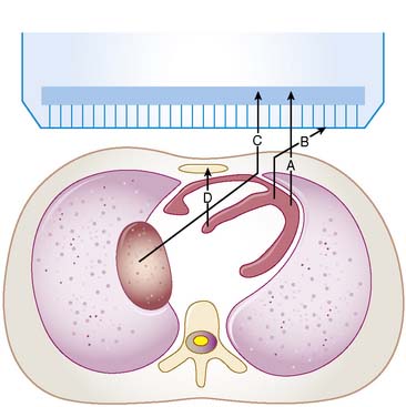
For a photon—whether gamma ray from technetium (^99mTc) or x-ray subsequent to the decay of thallium (²⁰¹Tl)—to become part of a cardiac image, it must first escape the body (see photon A in Fig. 6-1). The chances of this occurring are reduced in proportion to the likelihood that it will interact in the patient’s body before it can escape. At the photon energies of interest in nuclear cardiology, the major interactions in tissues are Compton scattering and photoelectric absorption.^8,9 In Compton scattering, a photon interacts with an electron that is loosely bound compared to the photon’s energy. The result of this interaction is the ejection of the electron from the atom and the creation of a new photon having a lower energy and different direction (see photons B and C in Fig. 6-1). The probability of interaction per unit path length (characterized by the linear attenuation coefficient for Compton scattering) depends on the tissue density and number of electrons per gram and decreases slowly with increasing photon energy. In photoelectric absorption, the photon imparts all of its energy to an electron, which is then ejected from the atom. The ejected photoelectron carries a kinetic energy that is equal to the energy of the incident photon minus the binding energy with which it was held to the atom. No scattered photon is emitted in the photoelectric interaction (see photon D in Fig. 6-1). However, characteristic radiation will likely be emitted when the electrons of the atom rearrange to fill the vacancy left by the photoelectron. The linear attenuation coefficient for photoelectric absorption increases as the cube of the atomic number of the atom, depends on tissue density, and decreases as the inverse cube of the photon energy.

Figure 6-1 Illustration of photon interactions of interest in patient for cardiac imaging. A, Transmitted photon originating in myocardium. B, Compton scattered photon originating in myocardium that collimator stops from striking crystal. C, Compton scattered photon originating in the liver that collimator allows to pass and results in the detection of an event that apparently originated in the myocardium. D, Photoelectrically absorbed in bone, which originated in myocardium.

Mathematically, the fraction of photons that will be transmitted through an attenuator or the transmitted fraction (TF) is given by:

(1)

where μ is the linear attenuation coefficient (sum of all the coefficients for individual interactions) and x is the thickness of the attenuator the photons pass through. If the attenuator is made up of a number of materials of various compositions, then the product μx in Eq. 1 is replaced by a sum of the attenuation coefficient for each material times the thickness of the material the transmitted photons pass through (path length the photons travel in the material). As a result of the differences in attenuation coefficient with type of tissue, the TF will vary with the materials traversed, even if the total patient thickness between the site of the emission and the camera is the same. Thus, one needs to have patient-specific information on the spatial distribution of attenuation coefficients (an attenuation map) to calculate the attenuation, which decreases the probability of photon detection.

Attenuation Artifacts (See Chapter 6)

The change in TF with direction of the photons and between different locations in the patient results in a variation in attenuation. This can be visualized in planar images as, for example, breast shadows and decreased counts in the presence of an elevated diaphragm. In SPECT slices, these artificial shadows are difficult to recognize; however, there is a pattern of altered relative counts consistent with the influence of attenuation in the mean bull’s eye polar maps of patients with a low likelihood of CAD. Eisner and colleagues reported decreased relative counts in the anterior wall of ²⁰¹Tl polar maps for females due to breast attenuation, and a relative decrease in the inferior wall of males, which may be due to diaphragmatic attenuation.¹⁰ The problem is that the location, extent, and severity of these reduced-count regions vary from patient to patient as a function of their anatomy. Thus, the variation in the pattern of apparent localization in disease-free patients is increased, resulting in more false-positive results (lower specificity) at any given level of true-positive results (sensitivity).

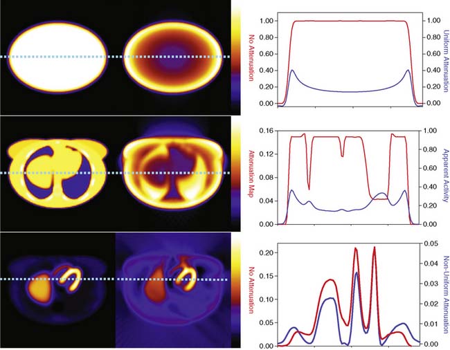
The types of changes in the reconstructed activity distributions when attenuation is present are illustrated in Figure 6-2. The top row of this figure shows what can be expected in the simple case of an elliptically shaped uniform-activity distribution without and with the presence of attenuation caused by a uniform attenuation distribution within the object. Note that attenuation causes a scaling of the reconstructed activity distribution such that there is a decrease by more than a factor of 2 at the outside, and a further decrease as one moves toward the center or most attenuated portion of the distribution. Hence an extended object that has a uniform distribution to begin with would have a loss in uniformity dependent on the relative depths of locations within it. The middle row of the figure shows the more complex case of a uniform source distribution that is attenuated by a non-uniform attenuation distribution simulating that of a cross-section through a female patient. This attenuation distribution and subsequent source and attenuator distributions the employed in the figures of this chapter were obtained from the mathematic cardiac-torso (MCAT) digital anthropomorphic phantom.¹¹ Notice that because the lungs have an attenuation coefficient approximately one-third that of soft tissue, there is now less attenuation within them than would have occurred had the entire cross-section consisted of soft tissues. Thus with attenuation, there appears to be a higher concentration of activity within them than the surrounding soft tissue, when actually the concentration was uniform. Notice also the sharp transition in apparent concentration of activity between the medial boundary of the lung and the heart region. The heart lateral wall is attenuated significantly more than the lung next to it. This explains why AC correction is very sensitive to having the correct registration between emission imaging and attenuation maps. A small movement can cause a big difference in the correction applied. The bottom row shows the even more complex case of both non-uniform source and attenuation distributions from the MCAT phantom simulating that of ^99mTc-sestamibi imaging. At the far left, in the absence of attenuation, the distribution of activity within the heart wall is uniform; however, when attenuation is included, a non-uniform distribution results, with the apex and lateral wall being brighter than the deeper lateral wall. Notice also that with attenuation present, there is now a mild change in the size and shape of the heart, as well as a significant distortion of the liver. With attenuation, there now is activity reconstructed as being outside the body. Such geometric distortion is greater for 180-degree reconstruction (as performed for these slices) than 360-degree reconstruction, owing to the greater inconsistencies in the emission profiles in the absence of their averaging by combining conjugate views.¹² The positive and negative tails from hot sources, which result from the incomplete cancellation of the inconsistent data in the emission profiles, can also lead to significant distortions in cardiac wall counts when there is significant extracardiac localization, such as with hepatic uptake. Germano and colleagues showed in phantom studies that an apparent reduction in counts occurs with the presence of a “hot” liver in the slices with the heart.¹³ Nuyts and colleagues¹⁴ observed that use of 360 degrees as opposed to 180 degrees with filtered backprojection (FBP) reconstruction reduced the magnitude of the artifact. The artifact was further reduced by use of attenuation compensation with maximum-likelihood expectation-maximization (MLEM) reconstruction.

Figure 6-2 Transverse slices showing examples of the distortion in apparent activity distribution caused by attenuation for (top) uniform activity and attenuation distributions, (middle) non-uniform attenuation and a uniform attenuation distribution, and (bottom) non-uniform attenuation and activity distributions. Top left shows a comparison of a slice through an elliptically shaped uniform-activity distribution and its reconstruction when attenuation is included in the creation of the SPECT data used in reconstruction. The attenuation distribution used to simulate attenuation during acquisition was also assumed to be uniform, with an attenuation coefficient equal to that of water for (^99mTc) photons. Notice that there is a significant decrease in the apparent activity in the reconstructed slice as one goes from the outside toward the center. The plots at the upper right are count profiles at the level indicated by the superimposed horizontal lines to the left for the original activity distribution (red) and the apparent distribution post reconstruction (blue). These graphically illustrate the impact of attenuation on the originally uniform activity distribution. Note that the scaling of the two count profiles is different, and that attenuation decreases the counts, even at the edge of the original distribution. Middle left shows a non-uniform attenuation distribution from the mathematic cardiac-torso phantom simulating that of a cross-section through a female patient, and the resulting apparent activity distribution when a uniform activity distribution is simulated as having been present in the patient. The outermost portion of the apparent distribution is again hotter, but now the lungs—which have a significantly lower attenuation coefficient than soft tissues—are also hotter. Note also the false presence of activity beyond the anterior surface of the body. Middle right shows overlaid plots of a horizontal profile through the attenuation map (red) and through the apparent activity distribution (blue), which clearly illustrate the impact of the less attenuating lungs. Bottom left shows 180-degree filtered backprojection reconstructed activity distribution that simulated that of ^99mTc-sestamibi imaging for the cases of first, no attenuation and then, use of the attenuation distribution of the attenuation map, shown in the middle row. Notice the loss of uniformity of activity distribution within the walls of the heart, the presence of activity outside the body, and the significant distortion of the liver, with the inclusion of attenuation when simulating the SPECT data. Bottom right shows count profiles at the level indicated by the horizontal lines of the slices, showing the increased non-uniformity in wall apparent uptake when attenuation is included during simulation of the SPECT data.

The artifactual decrease in apparent activity within the heart walls due to nearby extracardiac activity is further illustrated in the short-axis slices and circumferential count profiles at the top of Figure 6-3 for 180-degree reconstruction of Monte Carlo simulations¹⁵ of the MCAT phantom.¹¹ The top set of slices are with the liver uptake simulated as the same as that of the background. The next lower set of three slices shows the artifactual decrease in the inferior wall caused by the alteration of the liver activity to be the same as that of the heart. This alteration is illustrated graphically in the plots of the maximum count circumferential count to the right. There, one sees the typical pattern of a decrease in activity in the inferior versus the anterior wall due to the greater depth of the inferior wall, but this difference is dramatically accentuated by the increase in liver activity. This alteration in the apparent distribution of activity within the slices can be understood by the theory of the impact of attenuation on positron emission tomography (PET) and SPECT slices developed by Nuyts et al.,¹⁶ Bai et al.,¹⁷ and Bai and Shao.¹⁸ By this theory, attenuation causes a scaling of the counts at a given position, as illustrated in Figure 6-2, and a shifting of the local counts due to the attenuation of the other activity within the slice. It is this shifting that creates a negative bias that is the cause of the artifactual decrease in the inferior wall of the heart.

Figure 6-3 Comparison of Monte Carlo–simulated short-axis slices and circumferential profiles illustrating the impact of attenuation, attenuation correction (AC), and the inclusion of scatter. The two sets of three short-axis slices at the upper left show the uniformity of the activity within the LV wall when reconstructing 180 degrees of data using filtered back projection (FBP) without AC. The simulated acquisitions included the presence of non-uniform attenuation and camera distance-dependent spatial resolution but do not include scattered photons. In the first of these two sets, the concentration of activity within the liver was set to that of the background. In the second, it was set to be equal to that of the heart. Notice that the presence of a significant concentration of activity within the liver causes a significant apparent decrease in the inferior wall of the LV. This change is further demonstrated in the plots at the upper right, which show the maximum-count circumferential profiles from these short-axis slices. The middle of the five sets of short-axis slices shows the impact of using AC as part of maximum-likelihood expectation maximization reconstruction on the uniformity of the counts in the heart wall for acquisitions, with the liver activity concentration equaling that of the heart. The dramatic improvement in wall uniformity seen in the slices can be seen graphically by comparing the maximum-count circumferential profile plot for these slices at the lower right with those at the upper right for reconstruction without AC. The fourth set of three short-axis slices at the lower left illustrates the impact of the inclusion of scattered photons in imaging when the liver activity concentration is the same as in the heart. Notice that the apparent inferior-wall decrease seen without AC is now turned into an elevation in apparent inferior-wall counts with AC but no correction for scatter. This elevation is quantitatively demonstrated in the maximum-count circumferential profiles at the lower right. The bottom set of three short-axis slices is the reconstruction of solely the scatter contribution in the fourth set. Notice that scatter contributes to all regions of the slices, reducing wall contrast and apparent separation between the inferior heart wall and the liver.

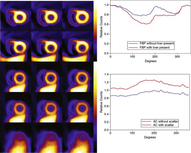
That AC, when included within iterative reconstruction, can correct this artifactual decrease as illustrated in the middle set of three short-axis slices at the left in Figure 6-3, and in the corresponding circumferential profile at the right. Notice that with AC, the wall now becomes fairly uniform in uptake. Notice also that the liver now becomes more intense than the heart, even though they were simulated as having the same concentration of activity. The reason for the apparent difference is the partial volume effect (PVE),⁹ which causes structures smaller in any dimension than two to three times the full-width-at-half-maximum (FWHM) measure of the system spatial resolution to be blurred such that their apparent activity is less than the actual value.

Broad Beam Attenuation and Scatter

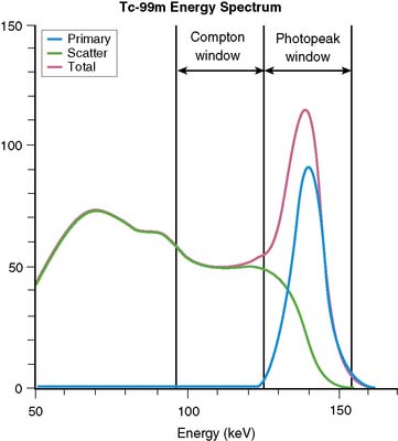
Equation 1 is accurate only (1) for a beam of photons with the same energy and (2) under the “good geometry condition” that, as soon as a photon undergoes any interaction, is no longer counted as a member of the beam.^8,9 Attenuation coefficients measured subject to these conditions are the “good-geometry” attenuation coefficients. Compton scattered photons, even though they are reduced in energy, are not necessarily excluded from being counted, owing to the finite width of the energy windows used because of the limited ability to distinguish different energy photons (finite energy resolution) of the cameras (Fig. 6-4). In fact, the ratio of scattered photons included in the energy window to primary photons in the energy window (scatter fraction) is typically 0.34 for ^99mTc¹⁹ and 0.95 for ²⁰¹Tl²⁰ for cardiac SPECT. Thus, Eq. 1 has to be modified to match the “broad beam” attenuation, which actually occurs in emission imaging by the inclusion of the buildup factor B, which is dependent on both μ and x. The result is^8,9:

Figure 6-4 Illustration of the energy distribution of primary and scattered photons for a technetium (^99mTc) point source in an attenuating medium. Shown also are the locations of the photopeak and Compton scatter windows.

(2)

Numerically, the buildup factor is the ratio between the sum of primary and scatter counts over the primary counts only, or the relative increase in counts due to the inclusion of scattered photons. It thus depends on variables such as location in the attenuator, geometry and composition of the attenuator, energy of the photon, energy resolution of the camera, and energy window used in imaging.

When scatter is not removed from the emission profiles before reconstruction, or its presence is incorporated into the reconstruction process itself, an overcorrection will occur. This is illustrated by the three sets of short-axis slices and the circumferential profiles at the bottom of Figure 6-3. As discussed previously, the top row of these slices illustrates how successful AC included within MLEM reconstruction can be at correcting the artifactual change in apparent uptake of the inferior wall of the row of slices just above it. However, the success of AC returning this slice to an apparent uniform concentration of activity within the walls is due in part to just primary photons being present. When the scattered photons acquired within the photopeak of the simulated acquisition are included, the short-axis slices next to the bottom are obtained. Notice how scatter has caused the inferior wall to now appear brighter than the anterior wall, which is the opposite of the effect of attenuation. The presence of scatter has also decreased wall contrast compared to the heart chamber region and visually decreased the separation of the heart from the liver. The bottom row of short-axis slices shows this is due to the non-uniform presence of scatter being concentrated closer to the liver. The circumferential profiles at the bottom right in the figure show that quantitatively, scatter has added approximately 30% more counts to the heart wall and that the inferior wall was increased the most.

Finite and Distance-Dependent Spatial Resolution

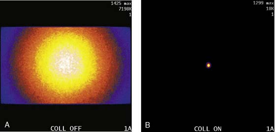
The third source of degradation discussed in this chapter is the finite, distance-dependent spatial resolution of the imaging system. When imaging in air, the system spatial resolution consists of two independent sources of blurring.⁹ The first is the intrinsic resolution of the detector and electronic components of the camera head. The second is the spatially varying geometric acceptance of the photons through the holes of the collimator. The collimator is the “lens” of the gamma camera; however, unlike optical lenses that form images by bending the light photons, collimators work by stopping all but the few photons that can pass through their holes without being absorbed by the septa of the collimator (absorptive collimation). This is illustrated in Figure 6-5, which shows two images of a very small point source of ^99mTc at the same location 10 cm from the detector face, first with no collimator and then with a low-energy high-resolution (LEHR) parallel-hole collimator on the camera head. The obvious need for the collimator is made clear by this figure, and so is the price paid for the use of the collimator in terms of loss in detection efficiency. Without the collimator, 7.2 million counts were collected in 1 minute. With the collimator, only 18,000 counts were collected in 1 minute, or 0.25% of that when the collimator was not on the system. The actual difference is greater because when the collimator was off, the count rate was near the maximum count rate of the system, so the recorded number of counts was depressed by resolving time count losses.⁹

Figure 6-5 Images of a (^99mTc) point source 10 cm in air from the face of the camera detector. A, No collimator on the camera head. B, Low-energy high-resolution collimator on the camera head.

As good as the image of the point source looks in Figure 6-5B compared to 6-5A, the ideal response would have been significantly better, since the point source was approximately only 1 mm in any dimension, and its bright representation in Figure 6-5B is larger than 10 mm across. The image resulting from imaging a point source of activity such as illustrated in Figure 6-5B is called a point spread function (PSF),⁹ and it portrays how a very small source of activity is blurred out during the course of imaging. Figure 6-6A illustrates plots through the center of Monte Carlo–simulated PSFs for an increasing distance of the point source in air from the face of a LEHR parallel-hole collimator. Notice how the PSF changes significantly in width and height as a function of distance. However, the area under the curves stays constant, consistent with no change in sensitivity with distance in air from the face of a parallel-hole collimator.

Figure 6-6 Illustration of the change in the spatial resolution with distance from the face of a low-energy high-resolution parallel-hole collimator for a (^99mTc) point source as depicted by the system point spread function (PSF), and the impact of this change in spatial resolution on one coronal slice through the heart and liver of the mathematic cardiac-torso (MCAT) phantom. A, Variation in Monte Carlo–simulated PSFs with distance for a point source in air (no contribution of scatter is included). Since sensitivity does not change with distance for a parallel-hole collimator, the area under all of the PSFs is the same. Thus, as the blurring becomes greater (the PSF wider), the maximum of the PSF decreases. This illustrates that increasingly lower fractions of the counts are left in place (not blurred) as one moves farther from the collimator. B, Coronal slices of the MCAT phantom. From upper left, the source distribution, upper right imaged as 10 cm distant in air from the face of the collimator, lower left imaged as 20 cm distant, and lower right imaged as 30 cm distant. Notice that as the distance away from the camera increases, the activity distribution is increasingly blurred, as exemplified by the heart and liver becoming increasingly smoothed together.

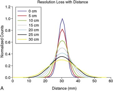
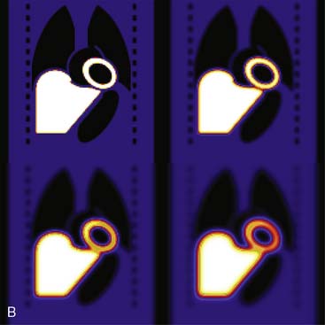
Figure 6-6B illustrates the impact of distance-dependent spatial resolution on one coronal slice through the MCAT phantom. As illustrated at the upper left in this figure, the concentrations of activity in the wall of the left ventricle (LV) and liver were the same, and that of the general tissue background was set to one-tenth that of the heart. All other organs had a concentration of activity of zero, as illustrated by the lungs, blood pool, and bones showing up as black. The slice at the upper right is that of the upper left blurred as if it were 10 cm from the face of a camera, as imaged with a LEHR collimator. The lower left slice is blurred as if acquired at 20 cm from the face of the collimator, and the lower right is 30 cm from the face. The FWHMs of the PSFs at these distances were 0.8 cm, 1.34 cm, and 1.88 cm. Notice how with increasing distance, the heart wall appears to become thicker and of apparently lower concentration relative to the liver. The apparent change in concentration is an illustration of the PVE or dependence of the apparent concentration of a structure on its size relative to the extent of blurring (FWHM).⁹ Note that the thickness of the wall in the slice varies due to the angulation of the heart relative to the coronal plane. Thus, the PVE causes the heart wall to appear as though it does not have a uniform concentration, when it actually had to begin with. Notice also that with increased distance, the liver and heart blur together to an increasing extent.