ECG Interpretation
4.1. A Systematic Method of Interpretation
The routine use of a systematic method of interpretation for both normal and pathologic ECG patterns as outlined below, is an effective way to avoid errors by ensuring that all shown parameters are checked. For example, the PR interval must be measured in the diagnosis of pre-excitation and AV block, while the QT interval is essential to the diagnosis of long and short QT syndrome.
Figures 2.29 and 2.30 show the temporal relationships between the different ECG waves and the names of intervals and segments.
4.1.1. Parameters for Study [A]
The parameters for studying normal and pathologic ECGs as the follows:
- Heart rate and rhythm.
- PR interval and segment.
- QT interval.
- P wave.
- QRS complex.
- ST segment and T and U waves.
- Calculation of the electrical axes of P, QRS, or T (ÂP, ÂQRS, ÂT).
- A normal ECG with no rotation of the heart and changes produced by rotations on the anteroposterior and longitudinal axes.
- The evolution of normal ECG with aging.
- Other normal ECG variants.
- A review of abnormal findings.
In this chapter we will comment on the normal characteristics of each of these parameters. This will be helpful when we look at the abnormalities affecting these parameters in the context of different pathologies.
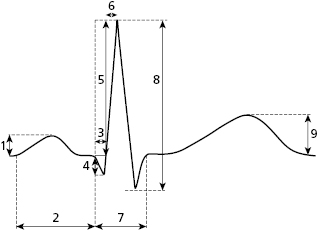
4.1.2. Measuring Waves and Intervals
Figure 4.1 shows how we measure the various waves, intervals, and segments described below.
4.2. Heart Rate and Rhythm
Figure 3.3B shows the distances between the vertical lines (voltage) and the horizontal ones (time). As previously described, the ECG recording device has to be calibrated, so that 1 cm in height equals 1 mV and a speed of 25 mm/s; the distance between two fine vertical lines (1 mm), corresponds to 0.04 s (40 ms); while the distance between two thick lines (5 mm) corresponds to 0.2 s (200 ms).
Using these calibrations, Table 4.1 shows a calculation of heart rate based on the RR interval.
Table 4.1 Calculation of heart rate according to the RR Interval
| Number of 0.20 s Spaces | Heart rate |
|---|---|
| 1 | 300 |
| 2 | 150 |
| 3 | 100 |
| 4 | 75 |
| 5 | 60 |
| 6 | 50 |
| 7 | 43 |
| 8 | 37 |
| 9 | 33 |
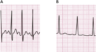
4.2.1. Characteristics of Sinus Rhythm [B]
Heart rhythm may be sinus or ectopic. Sinus rhythm is the rhythm of the sinus node, the structure with the greatest automatic capacity in the heart under normal conditions. The stimulus started in the sinus node spreads through the entire heart, originating the sinus P wave followed by the QRS complex and T wave. Nonsinus rhythms are known as ectopic rhythms and are discussed in the section on cardiac arrhythmias.
4.2.1.1. Characteristics of Sinus Rhythm
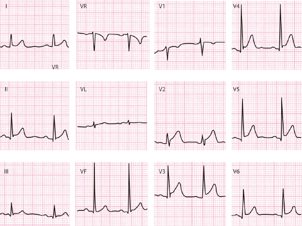
- The normal P wave is positive in I, II, VF, and V2-V6, and negative in VR. In III and V1 the normal P wave can be ±, and −+ in VL (Figs 2.6 and 2.25). In pathologic conditions it can be ± in II, III, VF, and V2–V3 (Fig. 5.6).
- The P wave is followed by a QRS complex with a normal PR interval (0.12 s to 0.2 s) in the absence of pre-excitation or AV block.
- The heart rate at rest is usually between 50–60 to 80–100 bpm and may present a slight irregularity in the RR intervals. In children this RR irregularity can vary and may even be evident, especially with breathing.
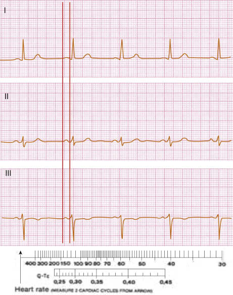
4.2.2. Measuring Heart Rate and the QTc Interval [C]
Heart rate may be measured according to Table 4.1. However, it may also be calculated, together with the corrected QT interval (QTc), using the rule shown in Figure 4.2 (see legend).
4.3. The PR Interval and the PR Segment
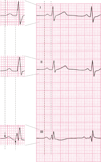
- The PR interval is the distance from the start of P to the start of QRS. The PR segment is the distance between the end of P and the start of QRS. To measure the PR interval correctly, a minimum of three leads must be used. This allows the interval to be measured from the lead where the P wave is first recorded to the lead where the QRS is first recorded (Fig. 4.3).
- The PR segment is generally iso-electric, but includes a part of the atrial repolarization wave that even under some normal conditions (sympathetic overdrive) may be seen (Fig. 4.4). In the context of pericarditis or atrial infarction, pathologic elevations or depressions in the PR segment are present and may help for diagnosis (Fig. 5.8).
- The normal duration of the PR interval in adults ranges between 120 ms and 200 ms.
4.4. The QT Interval
- The QT interval represents the sum of ventricle depolarization (QRS) and repolarization (ST-T).
- Sometimes it is not easy to measure. The best method is to trace a line extending the descending branch of the T wave until it crosses the iso-electric line (Fig. 4.5). This figure shows the method of measuring the QT interval in a 3-channel device. Note how the start of QRS begins in lead II.
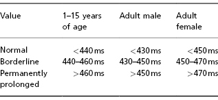
- It is necessary to correct the value of the QT interval in relation to heart rate (QTc). There are several formulas for this measurement, the most used being those by Bazett and Fredericia. However, in practice as we said, the calculation is made as is shown in Fig. 4.2. As a general rule, QTc should always be less than 430–450 ms (Fig. 4.2).
- Abnormalities in QT (long and short QT) may be hereditary or acquired and represent a risk of arrhythmia or even sudden death (see Chapter 16).
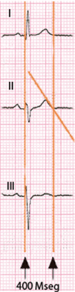
Table 4.2 QTc duration based on the Bazett formula in different age groups. Values are given in normal intervals, borderline, and abnormal intervals
4.5. P Wave [D]
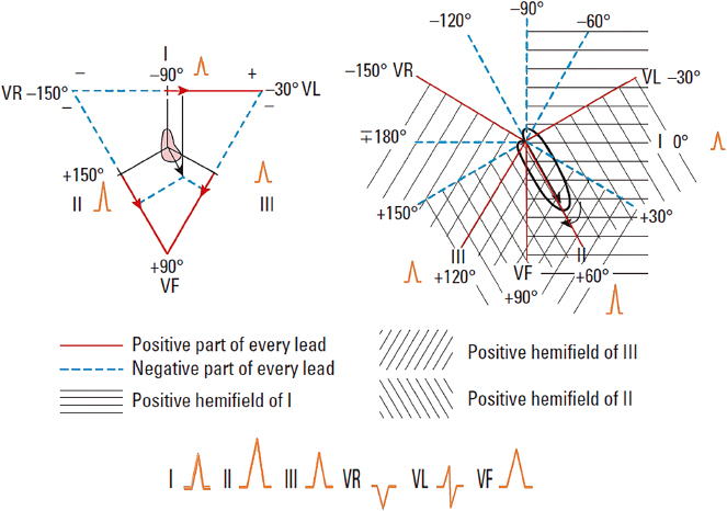
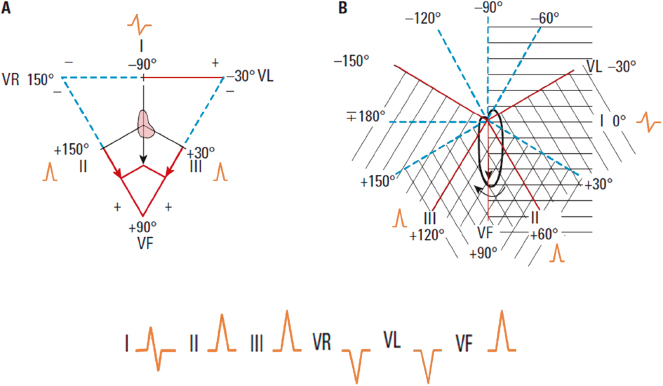
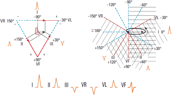
- The morphology of the P wave in different leads during sinus rhythm is described in Chapter 2. These morphologies appear according to the projection of the P loop in the respective hemifields of the leads (Fig. 2.25).
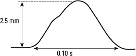
- Normal values for height and duration are 2.5 mm and <120 ms, respectively.
- Normal P wave height and width are measured as shown in Figure 4.6.
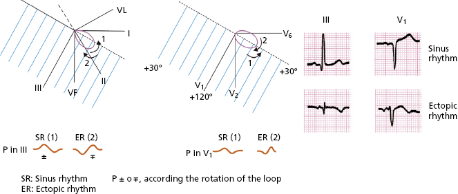
- Calculating the P axis (ÂP) is carried out as with QRS (ÂQRS) (p. 49). Under normal conditions (>90% of patients), ÂP ranges between +30° and +70°, and is never greater than +90° (negative P in lead I). This may only be seen in cases with electrode inversion, dextrocardia (right atrium on the left) or ectopic rhythm.
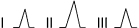
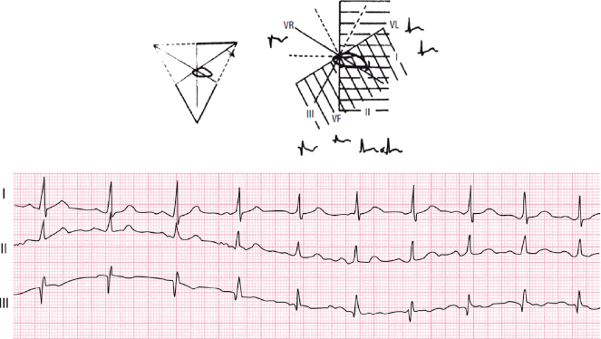
- A loop-hemifield correlation in cases of biphasic P wave (
 or
or  ) can determine whether the rhythm is sinus or ectopic (Fig. 4.7). Sinus rhythm in the P loop rotates counterclockwise in the FP and HP (Fig. 2.25).
 - A loop-hemifield correlation in cases of biphasic P wave (
4.6. The QRS Complex [E]
- The QRS complex is abrupt and normally presents two or three deflections (Fig. 2.29). Figure 4.1 shows how ECG parameters, including those of the QRS complex, are measured.
- The normal QRS morphology in a heart with no rotations may be seen in Figure 2.26, according to the loop-hemifield correlation.
- Figures 2.26 and 2.27 show how small changes in the loop-hemifield correlation can explain slight modifications in QRS in the FP leads.
- Normal values for voltage and duration in QRS are as follows:
- The width of a normal qRS should not exceed 100 ms.
- The voltage of the R wave should be no greater than 25 mm for V5-V6, 29 mm in lead I, and 15 mm in VL. However, some exceptions exist, especially in adolescent athletes and thin elderly individuals.
- The voltage in the q wave should not exceed 25% of that of the subsequent R wave, although some exceptions may occur in leads III, VL, and VF.
- The width of the q wave should be less than 40 ms and the recording should be abrupt.
- Low QRS voltage is defined by the sum of leads I, II, and II being less than 15 mm, or the sum of lead V1 or V6 as less than 5 mm, V2 or V5 as less than 7 mm, or V3 or V4 as less than 9 mm.
- The normal intrinsicoid deflection time (start of q to the peak of R) is less than 45 mm in V5-V6. This value may be greater in athletes and in presence of vagal overdrive, and sometimes in left ventricular enlargement.
- The calculation of the QRS axis (ÂQRS) is shown later (see Section 4.8). The normal value of this axis ranges between 0° and +90°, with a greater tendency toward 0° in the horizontal heart and a greater tendency toward +90° in the vertical heart. Ranges beyond +90° or +100°, or –20° or –30°, are considered pathologic.
- The width of a normal qRS should not exceed 100 ms.
4.7. ST segment and T Wave
4.7.1. The Normal ST Segment and Its Variations (Figs 4.9 to 4.13)
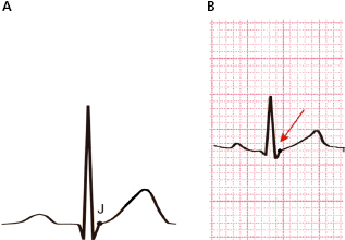
The ST segment is the distance between the end of QRS (J point) and the start of the T wave. Sometimes there is a notch (J wave) or slur (J wave type) at the end of QRS (see Fig. 16.14). Under normal conditions this segment is short with a slow slope going from the end of QRS until it reaches, usually with a slight elevation, the T wave forming with its ascending slope usually a curved line slightly convex respect to isoelectric line (Fig. 4.8). The ST segment is iso-electric at the start, or only slightly above or below the iso-electric line (no more than 0.5 mm ), except in V2-V3.In these leads may be elevated <2 mm in men (<2.5 cm in youngs) and <1.5 mm in women.
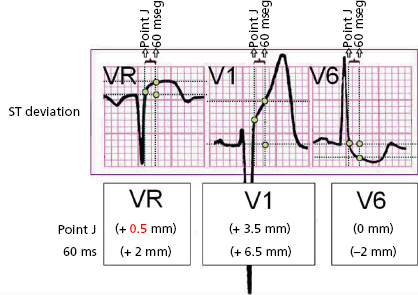
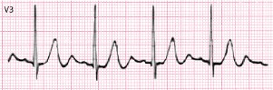
In vagal overdrive especially young persons, it may be elevated to 1-2 mm, or even more especially in mid/left precordial leads (Fig. 4.10B) as part of the typical early repolarization pattern, generally seen in V3-V5 (Fig. 4.10C) and less often in leads II, III, VF, I and VL.
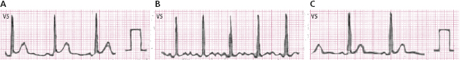
Occasionally, including in the absence of cardiomyopathy and especially in postmenopausal women or the elderly, it may be rectified or show a slight upsloping depression (<0.5 mm) (Fig. 4.10, E and F). In these patients it is useful to make a correlation with the clinical history (hypertension, precordial pain, etc.) and perform an exercise test to confirm the significance of this pattern. Figure 6.11 shows an example of normal ST slope (A), and a rectified one (B), in a patient with arterial hypertension.
Lastly, it may be elevated in V1-V2, in patients with pectus excavatum and rSr’ morphology (Fig. 4.10D). See the differential diagnosis with Brugada syndrome and other conditions in Chapter 16.
Figure 4.10 shows different ECG patterns that are seen in the absence of evident heart disease pattern. Some of these patterns are difficult to distinguish from pathologic ones.
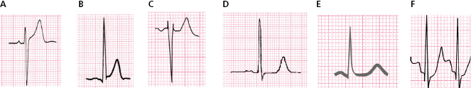
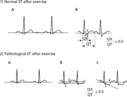
The ST segment can present a small depression in normal cases, somewhat with exercise or emotional state, but it rapidly slopes up thereafter (Fig. 4.11). The ST segment responds to exercise differently in normal individuals and patients with suspected ischemic heart disease. Figure 4.12 shows pathologic ST segment responses (see legend and Fig. 9.55).
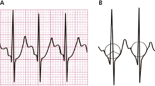
4.7.2. Measuring ST shifts [F]
The elevation and depression of the ST segment is measured either on the J point (end of QRS) or, at different levels (+20 to +60 ms) from it. The third universal definition of myocardial infarction advises measuring the ST shifts at the J point (Thygesen et al., 2012). Figure 4.9 shows how to measure shifts (ups and downs) of the ST segment, in this case an ST elevation acute coronary syndrome (STEACS). The elevation is measured from the upper border of the PR and the depression from the lower border. If PR is not iso-electric, it is measured from the level of the start of QRS (Fig. 4.12-2B).
4.7.3. The T Wave [G]
- The T wave is positive except in VR and sometimes V1, and sometimes flat or negative in III, VF, VL, and V2. Its voltage is lower, in general much lower than that of QRS. The T wave begins at the end of the ST segment (J point) with an upward slope that is slower than the downward slope (T wave asymmetry in general) (Fig. 4.8).
- The height of a normal T wave does not generally exceed 6 mm in the FP and 10 mm in the HP (middle/left leads), although in vagal overdrive and early repolarization it may reach 15 to 20 mm (Fig. 4.10).
- A high T wave in V1-V2, if symmetrical especially in V1, may be seen in the hyperacute phase of STEACS due to LAD occlusion (Fig. 9.16) and chronically in the case of lateral or inferolateral infarction (Fig. 9.38).
- A flat or negative T wave may be seen in specific clinical situations in ischemic heart disease (Chapter 9). It is usually not an expression of acute ischemia. It may appear:
- after the acute phase (post-ischemic T wave). Examples of this include cases of STEMI after percutaneous coronary interventionism (PCI), or fribrinolysis, or coronary spasm. In all these cases the T wave is very negative (Fig. 9.7);
- during a non-ST elevation ACS (NSTEACS). In these cases the T wave may be flat or only slightly negative) (≤2 mm) with RS or R pattern, sometimes even in leads morphology with rS; (Fig. 9.25);
- after Q wave-infarction: In this case the negative T wave corresponds to an intraventricular pattern (Fig. 9.30A).
- Figures 9.19 and 9.29 show other causes of high and sharp T waves and flat or negative T waves not related to myocardial ischemia.
- A high T wave in V1-V2, if symmetrical especially in V1, may be seen in the hyperacute phase of STEACS due to LAD occlusion (Fig. 9.16) and chronically in the case of lateral or inferolateral infarction (Fig. 9.38).
4.7.4. The U Wave
- A U wave may sometimes follow the T wave and have the same polarity but a lesser voltage.
- It is most commonly recorded in patients with bradycardia, especially those with advanced age, in leads V3-V5.
- If the polarity of the U wave is the opposite of the T wave, the cause is always pathologic (e.g. left ventricular hypertrophy, ischemia) (Fig. 9.27).
4.8. Calculating the Electrical Axis
The electrical axis is the resulting vector of the force generated by atrail depolarization (ÂP), ventricular depolarization (ÂQRS), and ventricular repolarization (ÂT).
The calculation of ÂQRS is explained below. ÂP and ÂT are calculated in the same way. We start at the ÂQRS located at +60° and we will see the projection of this vector on leads I, II, and III (A), and on the hemifields of these same leads (B). Later we will do the same with ÂQRS vectors located at right and left of +60°.
- ÂQRS +60° (Fig. 4.14)
With ÂQRS at +60° the QRS morphology is positive in leads I, II, and III, but with a higher voltage in II than in I or III (Figs 4.14 and 4.17) in accordance with Einthoven’s law: II = I + III.
- ÂQRS to the right = +90° (Fig. 4.15)
If we place ÂQRS at +90° the morphologies appear as shown in Figure 4.15 in accordance with that shown in Figure 4.14.
- ÂQRS to the left = 0° (Fig. 4.16)
If we place ÂQRS at 0°, the morphologies in the FP appear as shown in Figure 4.16 in accordance with that shown in Figure 4.14.
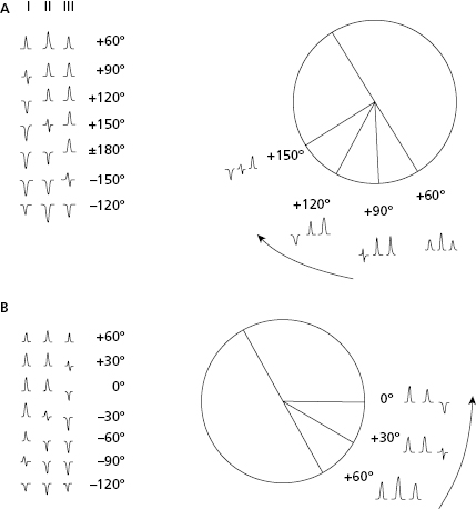
- Calculating ÂQRS in practice (Fig. 4.17) [H]
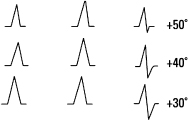
- ÂQRS (and ÂP as well as ÂT) may be calculated in practice using the QRS morphologies in leads I, II, and III bearing in mind that ÂQRS at +60° has positivity in all three leads, with II equaling the sum of I and III.
- We then have to add or take away 30° for each change of morphology from positive to isodiphasic or from isodiphasic to negative. Thirty degrees are added if a change starts in I, in which case the morphology changes in I before than III. Thirty degrees are taken away if the change is initiated in III (Fig. 4.17).
- To obtain a more precise calculation for intermediate values of ÂQRS, we must proceed to the process explained below.
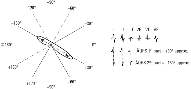
- Indeterminate ÂQRS (Fig. 4.18)
When isodiphasic QRS complexes occur in I, II, and III the vectorial forces do not have a predominant direction and a GLOBAL ÂQRS cannot be calculated, although the first and second parts may be determined as shown in Figure 4.18.
- The value of measuring ÂP, ÂQRS, and ÂT
The importance of measuring these axes will become more and more apparent throughout this book, especially in the diagnosis of cavity enlargement and ventricular block. It has been recently shown that the angle formed by ÂQRS and ÂT in the frontal plane is a useful prognostic marker (see Bayés de Luna, 2012a). - Calculating ÂQRS in practice (Fig. 4.17) [H]
4.9. Heart Rotation and Its Repercussions on the ECG
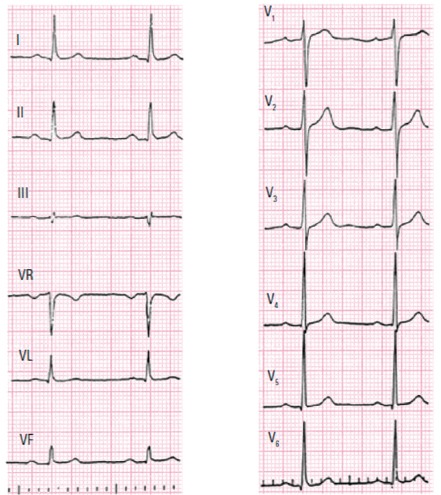
4.9.1. The Normal ECG with no Rotation
- A heart with no rotation (intermediate heart) presents a ÂQRS located at about +30° and transition from the right ventricle to the left ventricle (qRs) starts in V4-V5, generally with a qR morphology (or qRs) in V6 (Fig. 4.19).
- However, a normal heart often presents some rotation on the anteroposterior and longitudinal axes which modifies the ECG; we are aware of this, but it does not indicate pathology. In different heart diseases we may see ECG patterns that are due to underlying heart disease associated or not to some rotations of the heart.
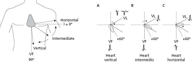
4.9.2. Heart Rotation on the Anteroposterior Axis (Fig. 4.20) [I]
The normal heart often presents a rotation on the anteroposterior axis. This originates a verticalization or horizontalization of the heart that is especially visible in the FP (VL and VF) (see Figure 4.20 and legend).
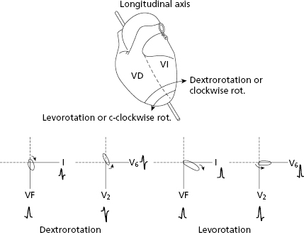
4.9.3. Heart Rotation on the Longitudinal Axis (Fig. 4.21) [J]
Rotation of this axis originates a levorotation or a dextrorotation that is especially visible in the HP (V2 and V6) (see Fig. 4.21 and legend).
4.9.4. Combined Rotations (Fig. 4.22)
The vertical heart is often dextrorotated and the horizontal heart is often levorotated (Bayés de Luna, 2012a). A combined rotation, which is important to understand to avoid confusion with an inferior infarction, because in both cases may be Q in III, is the dextrorotated but horizontralized heart. The QRS loop rotates clockwise in the FP, but is oriented between 0° and 20°. This causes an SI Q3 morphology that disappears with breathing (change from Qr to qR). This is explained because the heart changes to a semivertical position and the loop is oriented at ≈50°) (Fig. 4.22).
4.10. Variations of Normal ECGs
4.10.1. Normal ECG Changes with Age
- Children (Fig. 4.23) [K]
- Faster heart rate
- ÂQRS is usually to the right
- R voltage in V1 is greater than q in V6
- Infantile repolarization. See Fig. 4.23.
- Adolescents occasionally show high voltage in precordial leads without left ventricular enlargement in the echocardiogram.
- Sometimes
 is recorded in V1 in children. This pattern is modified with breathing (see Bayés de Luna 2012a).
- Faster heart rate
- The elderly (Fig. 4.24) [L]
- Greater incidence of sinus bradycardia.
- ÂP generally >60°. Therefore PI < PIII.
- ÂQRS more to the left (0° or more).
- Longer PR interval (up to 0.22 ms).
- Frequent dextrorotation (evident S wave in V6) due to emphysema.
- Generally lower QRS voltage. Occasionally increased voltage, especially in thin individuals.
- Sometimes ST rectification or even small ST depression.
- Sporadic isolated extrasystole.
- Greater incidence of sinus bradycardia.
4.10.2. Transitory Changes in Repolarization
A flattened T wave may be seen in healthy individuals following hyperventilation (Fig. 4.25), alcohol or glucose consumption, etc.
4.10.3. Other ECG Patterns in the Normal Heart
S1, S2, S3 pattern. This morphology may be seen in the normal heart, but also in right enlargement and peripheral right bundle branch block (Chapters 6 and 7).
Early repolarization (ER) pattern. This morphology presents an abrupt wave (J wave) or slurrings at the end of QRS that is generally combined with some ST elevation. It occurs in 2% of the population, especially in the middle and left leads, often in athletes and in presence of vagal overdrive. It has been associated with the appearance of primary ventricular fibrillation (VF) (Haïsaguerre, 2008), especially when it appears in inferior leads. However cases of ER (Fig. 4.26) are not considered dangerous except in very specific circumstances, such as the presence of J waves greater than or equal to 2 mm in inferior leads (Fig. 16.14) or abrupt voltage changes of this wave or if are followed by horizontal or descending ST segment. Furthermore, we have to be sure, in analogic not digital recording, that this pattern is not due to a recording artifact (Fig. 3.7). [M]
Other changes related to gender or race exist, but are usually non-significant (see Bayés de Luna, 2012a).
4.10.4. Repeat the ECG Recording If an ECG Pattern Is Unusual
For instance, negative P wave in lead I; qR pattern in lead V2 with rS in V1 and RS in V3, and QR pattern in lead III. Check the recording errors and record the ECG during deep inspiration in case of QR in lead III (see Section 3.3 in Chapter 3, and Figure 4.22).
Self-assessment
A. List the study parameters in an ECG recording.
Stay updated, free articles. Join our Telegram channel

Full access? Get Clinical Tree


