The ECG Curve: What Is It and How Does It Originate?
2.1. How Does the TAP of a Myocardiac Cell Become the Curve of the Cellular Electrogram?
The electrical activity (depolarization and repolarization) of a contractile cell (or wedge preparation) is recorded when a microelectrode is located outside the cell and another inside, as a steep positive curve followed by a plateau with a descending slope, called the transmembrane action potential (TAP) (see Figs 2.1A and 1.6).
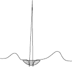
However, if the deflection of this electrical activity is recorded by an electrode located on the opposite side of the cell (or wedge preparation), it shows one curve, called the cellular electrogram, formed by a sharp, high-voltage positive wave (QRS) ( ) followed by an isoelectric space, and then a more gradual, wide negative wave with a lower voltage, known as the T wave (
 ), results (Fig. 2.1). [A]
We will now look at the formation process of the cellular electrogram curve (Fig. 2.1B and C) (see Bayés de Luna, 2012a; Macfarlane et al., 2011).
2.1.1. The Formation Process of the Cellular Electrogram (Cellular Activation) (Fig. 2.1)
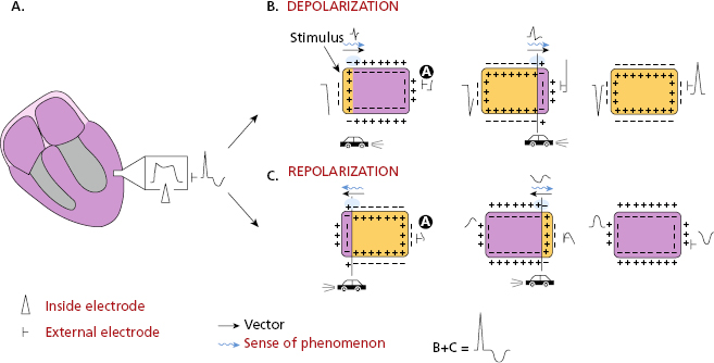
2.1.1.1. Cellular Depolarization (Fig. 2.1B)
When a cell (wedge preparation) is activated, it receives an electrical impulse and depolarizes. During this phenomenon the surface of the cell that was full of positive charges becomes negative, starting in the place where the stimulus is applied, with the formation of a dipole of depolarization that is a pair of charges, namely, −+. This dipole advances along the surface of the cell to the area where the electrode is located, that is on the opposite side. The depolarization dipole has a vectorial expression, with the head of the vector located on the positive side of the dipole. [B]
As it advances, a progressively more positive deflection is detected, until finally it is completely positive ( ) (equivalent to QRS complex). An electrode located in the central part of the cell records first positively and later negatively (
 ), because it first faces the head of the depolarization dipole (head of the vector), and then the tail of the vector, which is negative.
2.1.1.2. Cellular Repolarization (Fig. 2.1C)
Once the cell (or wedge preparation) is depolarized, the process of repolarization takes place. This process starts by means of the repolarization dipole (+−), originating on the same side as the depolarization dipole. The repolarization dipole advances in the surface of the cell and progressively recovers the lost positive charges, slowly reaching the recording electrode, producing a slow and gradual negative curve (T wave). [C]
Cellular activation may be compared to a car passing by in the dark, going towards the recording electrode. The lights of the car, as it moves closer, are facing the electrode which records positivity (depolarization). Afterwards, the car starting from the original point advances in reverse towards the same electrode. However, as the car approaches the electrode, because the lights are facing the opposite side, it records negativity (repolarization) (Fig. 2.1B and C).
2.1.2. Why Is the T Wave in the Human ECG Positive, While in the Cellular Electrogram It Is Negative?
This may be explained by two theories.
2.1.2.1. The Theory of the Depolarization and the Repolarization Dipole (Fig. 2.2)
If we look at the left ventricle, which is responsible for the human ECG to a large degree, acting as an enormous cell, it is possible to see how depolarization starts in the endocardium, where the electrical stimulus arrives from the Purkinje fibers. An electrode (├ A), located on the epicardium on the opposite side, meanwhile detects that the depolarization dipole is approaching; this is a positive complex because this electrode faces the positive charge of the depolarization dipole (the vector head).
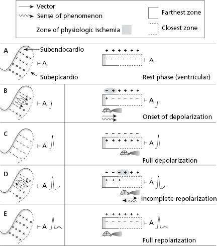
However, repolarization does not begin in the same location as that of the isolated cell. Repolarization in the heart begins in the most perfused area: the subepicardium. The subendocardium is an area of terminal perfusion, and physiologically it is less perfunded than the subepicardium. The subendocardium may be considered to have some physiologic ischemia. Thus the repolarization dipole advances from the subepicardium to the subendocardium, like a car passing by in reverse with the front lights visible (positive charge of the dipole, or vector head), facing the subepicardium. Thus a positive charge is detected there. [D]
In summary: The path of the electrical activity in the LV of the human heart is determined by depolarization and repolarization dipoles as previously described. These dipoles have a vectorial expression, with the head of the vector located at the positive charge.
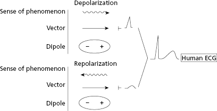
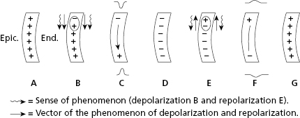
Figure 2.3 outlines the sense ( ) of the depolarization and repolarization phenomenon, the dipoles, and its vector
  expression during depolarization and repolarization (activation) of the heart, namely of the LV, which is considered to be mostly responsible for this process.
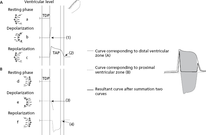
2.1.2.2. The Theory of the Sum of TAP of the Subendocardium and Subepicardium
This is an alternative theory that may explain the formation of a human ECG curve. The human ECG recorded from an electrode (├) located on the LV epicardium (largely responsible for the ECG curve) may be considered, according to Ashman (Bayés de Luna, 2012a), the sum of the TAP of the subendocardial area and the TAP of the subepicardial area of the LV wall. As the TAP of the subepicardium is recorded as negative and starts and ends before the TAP of the subendocardium, which is recorded as positive, the sum of both explains the recording of a positive deflection (QRS), an isoelectric space (ST) and a terminal positive wave (T) (see legend, Fig. 2.4). [E]
2.2. The Activation of the Heart
- Only activation (depolarization and repolarization) of the atrial and ventricular myocardial mass (contractile cells) is detected in the ECG (P QRS-T).
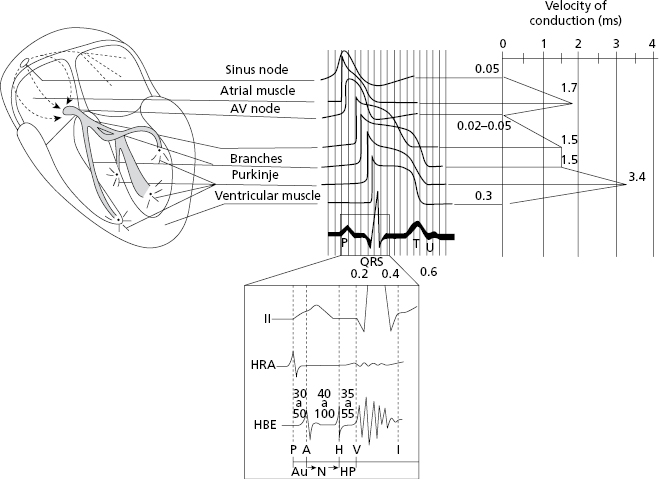
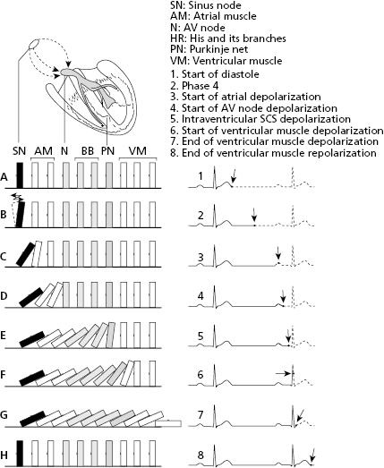
- The electrical activation of the sinus node (SN) and the passing of the stimulus through the SCS are not recorded on a surface ECG, because the electrical potential they generate is too low. The lower part of Figure 2.5 shows how these potentials may be detected as short, sharp deflections in a recording of intracavitary ECG.
- Figure 2.5 shows the correlation between the action potential (TAP) generated by cells in specific areas of the heart and the surface ECG, as well as the stimulus conduction speed as it passes through these areas.
- The global depolarization vector of the atria (P wave) and ventricles (QRS) is the sum of many successive, instantaneous depolarization vectors in these structures, configuring the P and QRS loops (see below) (Figs 2.6 and 2.9).
2.2.1. Atrial Activation (Fig. 2.6)
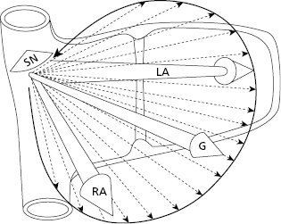
Atrial depolarization (Figs 2.6 and 2.7) begins in the SN and goes first to the right atrium, spreading in concentric curves to the septum and left atrium mainly through the Bachmann bundle. [F]
The sum of multiple instantaneous vectors in the atria originates a curve called the atrial depolarization loop, which represents the path followed by the stimulus following depolarization of both atria. Due to the fact that this begins in the right atrium, it follows a spatial anti-clockwise direction. This atrial depolarization loop can express itself with a maximum or global vector, that is the sum of all instantaneous atrial depolarization vectors and, ultimately, the sum of the depolarization vectors of the right and left atria. The positive part of the atrial depolarization global dipole is located at the head of this global vector. Thus, on the surface of the body (left thorax) a positive curve, called the P loop or wave, is recorded.
Depolarization of atrial muscle, which has a very thin wall, starts in the SN and continues along the entire wall. When depolarization begins, a depolarization dipole with a vectorial expression forms, and is directed toward the electrode located in front, originating a positive wave (P wave) (Fig. 2.7A and D).
Atrial repolarization (Fig. 2.7E to G) begins in the same place (E) as depolarization, and the repolarization dipole also occupies the entire thickness of the atrial wall because, as stated previously, this is very thin. Consequently, the repolarization dipole approaches the recording electrode (left thorax), which faces the negative charge of the dipole (vector tail), resulting in the recording of a slower and longer negative curve compared to the positive P wave because the process is more lasting (F and G).
The negative wave of atrial repolarization is not generally detected, because it remains hidden in the ventricular depolarization complex (QRS) (Fig. 2.8), except when the P wave has a high voltage or when AV block occurs, which produces a delayed recording of QRS.
2.2.2. Ventricular Activation
The path of the stimulus through the intraventricular SCS is recorded in the ECG as a straight line between the atrial activation P wave and the ventricular activation (QRS-T), and this corresponds to the PR segment.
The electrical stimulus reaches three areas of the LV first (Fig. 1.3D). These areas correspond to the superoanterior and the inferoposterior fascicles, and the middle fibers (also named septal fascicles).
Ventricular depolarization: The path of the electrical activity through the ventricles, from the endocardium to the epicardium, originates a loop (Fig. 2.9A) that when recorded with an electrode located in front of it in the LV epicardial wall, may be divided into three vectors. The middle vector, or vector 2, is the most important and is the expression of most of the depolarization of the LV (R wave). An initial part, vector 1 (q wave), moves from left to right, and upwards in the intermediate and vertical heart (in the horizontal heart below), and represents the sum of the depolarization of the three small areas of initial depolarization in the LV as described by Durrer (Fig. 1.3D). Lastly, vector 3 represents the depolarization of the last parts of the septum and the right ventricle (RV) and it is also directed upward and to the right (‘s’ wave). By joining these three vectors, we have a loop that represents the whole of the ventricular depolarization process known as the QRS loop or QRS complex. [G]
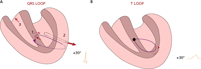
The QRS loop in Figure 2.9A is that of a heart in an intermediate position with a morphology that is detected with an electrode (├) located in front of the main depolarization vector (vector 2) (see Figs 2.11 and 2.26).
Ventricular repolarization takes place later on, the path of which explains the formation of a loop (T wave or loop) with a maximal vector similar to the QRS global loop (Figs 2.9B, 2.11, and 2.28).
Naturally, the QRS and T loops, at different rotations of the heart, vary according to the different locations of the vectors and the orientation of the loops (Bayés de Luna, 2012a).
2.2.3. Domino Theory
Cardiac activation can be compared to a row of dominoes as they fall. Sinus node, with the most automatic capacity (black domino), corresponds to the first domino, transmitting the stimulus to the neighboring structures. Figure 2.10 shows each phase, from the start of the diastole (phase 1), through all diastole (DTP) (phase 2), and then the entire activation phase (depolarization and repolarization of the atria and ventricles, phases 3 to 8). The grey dominos show decreasing automaticity. [H]
2.2.4. Cardiac Activation Summary: Dipole, Vector, and Loop and Their Projection on the Frontal and Horizontal Planes
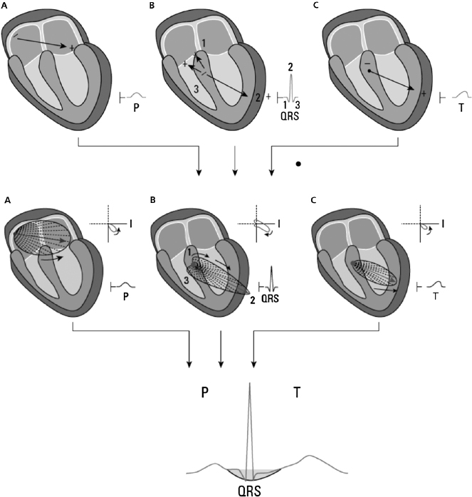
Figure 2.11 shows how the sum of the atrial (A) and ventricular (B) depolarization vectors and ventricular repolarization (C) (top), with the corresponding loops (middle) can explain the morphology of an ECG taken from an electrode (├) on the surface of the LV. Positivity is recorded when the electrode faces the head of the vector and negativity when facing the tail, regardless of whether the phenomenon is moving towards (depolarization) or away from (repolarization) the recording electrode. Obviously, an electrode located opposite to this location will record an inverse pattern (Figs 2.11 and 2.12).
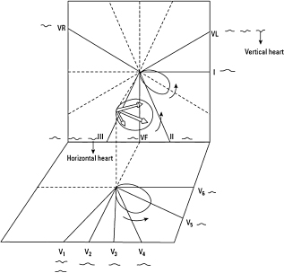
2.2.5. The Projection of the Electrical Activity of the Heart on a Plane Surface
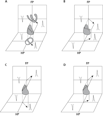
Bearing in mind that the heart is a three-dimensional organ, visualizing on paper or screen the electrical activity of the heart (vector or loop) must involve two planes, the frontal plane (FP) and the horizontal plane (HP).
Figure 2.12 shows how the projection of different spacial vectors (or loops) originate positive or negative morphologies on the FP and HP according to whether the location of the recording is facing the head (+) or tail (–) of this vector.
Even before we examine specific derivations or the projection of vectors and loops in the positive and negative hemifields of these derivations, it is possible to see that positivity or negativity is recorded according to whether we face the head or tail of the vector. The projection of loops on the FP and HP that will be explained later, will clearly explain why bi or trifascicular deflections are recorded.
2.3. Lead Concept
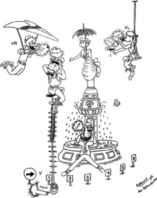
To see better landscapes, monuments and sculptures on a plane surface, we must take pictures from several angles, as seen in Figure 2.13. In the same way, to understand better the electrical activity of the heart, we have to record the ECG from various points, called leads. The ECG morphology differs according to the location from which the recording takes place. [I]
There are six leads located on the frontal plane (FP): I, II, III, VR, VL and VF. They record the electrical activity with electrodes located on the limbs. There are also six leads on the horizontal plane (HP): V1-V6, which record this activity with electrodes placed on the precordium (see below).
Each lead is placed in a specific place (at an angle) on the FP of HP, and each lead has a lead line that travels from the opposite side (180°) passing through the center of the heart. Each lead is also divided into positive and negative parts. The positive part goes from the point in which the lead is located to the center of the heart (a continuous line, in Figures 2.14 to 2.18). The negative part is made up from the center of the heart to the opposing pole (discontinued line, Figs 2.14, 2.15 and 2.18).
2.3.1. Frontal Plane Leads
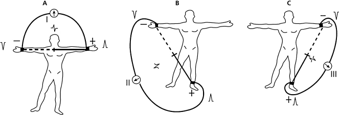
There are three leads called bipolar limb leads located between two points of the body (I, II, and III) (Fig. 2.14) and three monopolar leads (VR, VL, and VF), which are in fact also bipolar because they measure the difference in potential between a point (VR on the right shoulder; VL on the left shoulder and VF on the left leg) and the central terminal connected to the center of the heart (Fig. 2.16). [J]
The three bipolar leads of the limbs are recorded through electrodes located on the arms and legs. Lead I (A) obtains the difference in potential between the left arm (+) and the right arm (−), lead II (B) between the left leg (+) and the right arm (−), and lead III (C) between the left leg (+) and left arm (−) (Fig. 2.14).
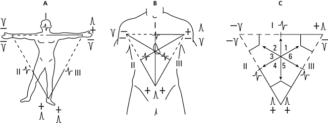
These three bipolar leads constitute the Einthoven triangle, shown in Figure 2.15A. Figure 2.15B shows the triangle superimposed on the human torso (B). We can see the positive part (continuous line) and the negative part of each lead.
Different vectors (1 to 6) (Fig. 2.15C) originate different projections according to their location. For example, vector 1 has a positive projection in lead I, a negative projection in lead III, and an isodiphasic (0) in lead II. Thus, the voltage of lead II is equal to the sum of the voltages of I and III.
This sum, II = I + III, is called the law of Einthoven. This law must always be observed in order to ensure that the ECG is recorded and labeled correctly.
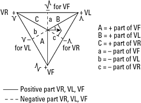
Leads VR, VL, and VF record the electrical activity from the right shoulder, the left shoulder, and the left leg. They also have a lead line with a positive part, which goes from the recording point to the center of the heart (continuous line) and a negative part that goes the area from the center of the heart to the opposite point (dotted line).
Any vector projected in VR, VL, or VF originates a projection that may be positive, negative, or isodiphasic. In Figure 2.16, vector 1 directed at 0°, has a positive projection in VL (B  ), a negative projection in VR (C
  ) , and an isodiphasic projection in VF (
 ).
).
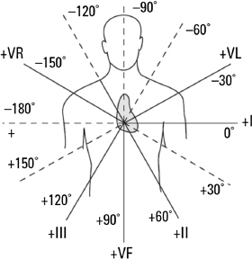
Bailey hexaxial system (Fig. 2.17): If we move the three leads of the Einthoven triangle, I, II, and III, to the center of the heart, we see that they are located at +0° (I), +60° (II), and +120° (III). If we do the same with the three leads VR, VL, and VF, they will be located at VR (−150°), VL (−30°), and VF (+90°). This situation constitutes the Bailey’s hexaxial system in which all the distances among the positive and negative lead lines of all six leads of the FP are separated by 30°.
These spacial references among the FP leads, and also to those of the HP (see later), must be memorized. While this book is meant for deductive teaching, there are some concepts that must be retained in one’s memory.
2.3.2. Horizontal Plane Leads
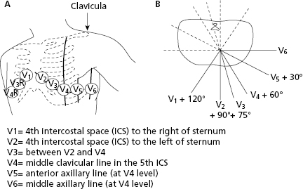
Figure 2.18 shows where the electrodes of the six precordial leads on the thorax are located (A) and the angles of the six positive poles with the separations existing between them (B). Figure 2.18 explains in detail where these six leads should be correctly placed. This is extremely important because the ECG morphologies may be modified, especially in V1–V2, with small changes in location, causing potentially dangerous confusion (see Sections 3.2 and 3.3 in Chapter 3). [K]
Occasionally, recordings of leads in the right side of V1 (V3R, V4R) (Fig. 2.18) or the left of V6 (V7: posterior axillary line; V8: inferior angle of scapula; and V9: left paravertebral area) are made. These may be useful in some cases of ischemic heart disease (Chapter 9), but they are not used much in practice.
2.4. Hemifield Concept
If we trace to each lead a perpendicular line that passes through the center of the heart, we will obtain one positive and one negative hemifield. [L]
Figure 2.19A shows how in leads I and VF the corresponding vector and loop fall in the positive hemifield of each lead, and thus the morphology in both is completely positive. In Figure 2.19B and C we may see how an ECG morphology in a lead, in this case VF or I, can be +− or −+, with the same maximal vector direction, according to whether the rotation of the loop is clockwise (a) or anti-clockwise (b). In addition, Figure 2.19D shows how the start and end parts of QRS originate through the correlation of this part of the loop with the positive or negative hemifields (I and VF in D).
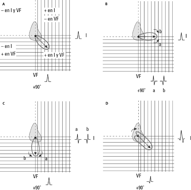
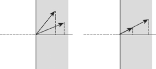
Figure 2.20 shows how voltage of a vector or loop is of greater or lesser importance in different leads according to the magnitude and direction of this vector or its corresponding loop, in this case in lead I. Where there are two vectors with the same direction, the voltage in this lead will only depend on the magnitude of the vector (B). However, in case of vectors with the same magnitude (A) the voltage in this lead depends on the location of the vector in its positive or negative hemifield, and consequently on the projection of this vector on the corresponding line of the lead, in this case lead I.
If a vector (Fig. 2.21) falls in the positive or negative hemifield of a particular lead, it originates a positivity or negativity in this lead. If it is located at the limit of both hemifields, the deflection will be diphasic +− or −+, according to the clockwise or counter-clockwise sense of the loop (see Figs 2.19, 2.22–2.24).
2.4.1. Vector–Loop–Hemifield Correlation
By considering loops (global stimulus path) instead of the maximal vector, which does not include the direction of stimuli and the presence of initial and final vectors, we are able to understand the following: (1) in cases of maximal vector that falls in the limit of a positive and negative hemifield of a lead, whether the morphology will be  or
or  , according the sense of rotation of the loop; and (2) how to explain the positive or negative initial and/or final parts that many complexes present (
 ,
,  ). [M]
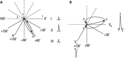
This loop–hemifield correlation in a normal heart with a QRS loop and a maximal vector located at +60° in the FP and −20° in the HP explains the morphology recorded in these leads (Fig. 2.22).
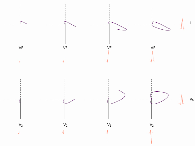
Figure 2.23 explains how the ECG morphology allows us to estimate the stimulus path, that is the P, QRS, or T loop (in this case QRS), and vice versa. The morphologies in two leads are always correlated with the corresponding loop and vice versa; in Figure 2.23, VF and I, and V2 and V6. In this figure, in lead I and VF, firstly a small negative deflection is recorded. This indicates that the loop begins in the negative hemifield of both leads, but soon moves first toward the positive hemifield of lead I, because positivity is recorded in this lead first. Next, it enters in the positive hemifield of VF, but the initial negativity (q) in I is lower than in VF, because the greater part of the loop is in the negative hemifield of VF than of I. Finally, the QRS complex ends with a small negativity in I, but not in VF, indicating that the loop has completed its path and upon closing remains in the positive hemifield in VF and somewhat in the negative hemifield of I.
The same process in reverse produces a recording of the ECG curve through the loop. For the loop–hemifield correlation in V2 and V6 we can follow the same rule.
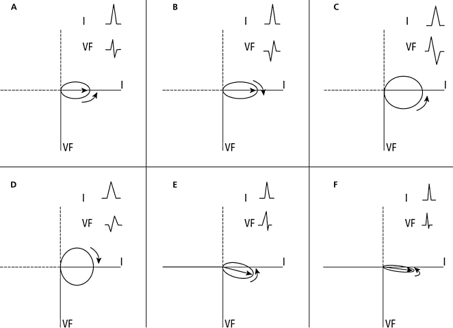
Figure 2.24 shows an isodiphasic deflection in a specific lead (in this case VF) that can be positive–negative (A) or negative–positive (B) according to the sense of rotation (clockwise or counter-clockwise of the loop). The area of the complex is greater if the loop is more open (C and D). Lastly, if a large part of the loop is located in the positive hemifield, the deflection is diphasic, but not isodiphasic (E and F).
2.4.1.1. Loop-Hemifield Correlation: P Loop (Fig. 2.25)
Figure 2.25 shows the P loop in a heart without rotations and its projection on the FP (maximal vector at +30° in EF) and the HP. The loop–hemifield correlation explains the morphology of the P wave in the 12 leads and the changes that may be produced in cases of a heart with vertical or horizontal position (see Chapter 4). [N]
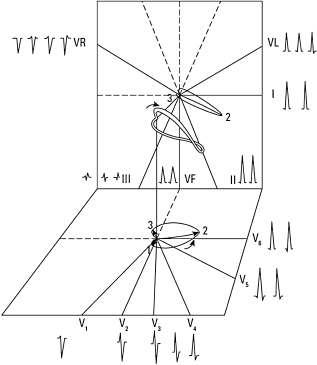
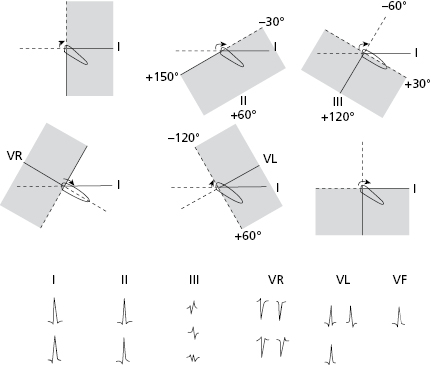
2.4.1.2. Loop–Hemifield Correlation: QRS Loop (Fig. 2.26)
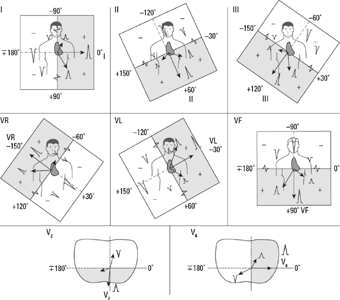
This figure shows the projection of the QRS loop in the FP and HP in a heart without rotations (intermediate position and maximal vector +30° in FP), as well as the QRS morphology in the 12 ECG leads, according to the loop–hemifield correlation (see Chapter 4). The different QRS morphologies in the six FP leads according to the projection of the QRS loop on the positive or negative hemifield of each lead can be seen in more detail in Figure 2.27.
2.4.1.3. Loop–Hemifield Correlation: T Loop (Fig. 2.28)
The projection of the T loop on the positive and negative hemifields of the 12 leads explains the T wave morphology. Small changes in the orientation of the loop can change the morphology, especially in V1–V2, III, VF, and VL.

Full access? Get Clinical Tree


