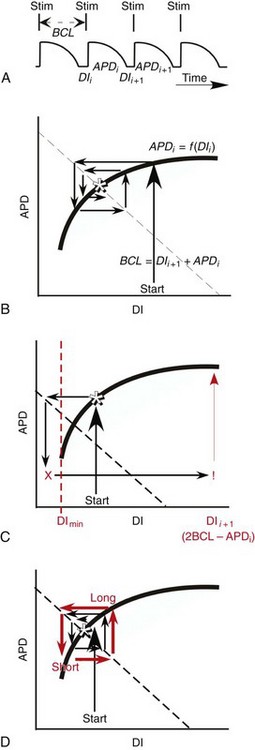
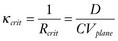
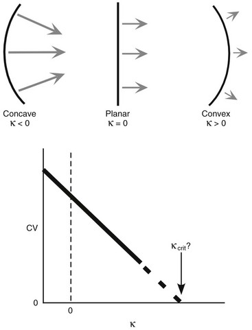
34 Since the landmark publication of Gordon Moe’s multiple wavelet hypothesis,1 it has been assumed that heterogeneity of the refractory period is an essential element of VF. Only in the past two decades (much longer in Russia) has it become clear through theory and mathematics, as well as by counter-examples in numerical experiments, that reentry can occur in tissue with homogeneous refractoriness. Rotors form as a result of regional conduction block of an action potential wave propagating within the heart; this block can arise via static or functional heterogeneities (or a combination of both). I restrict myself to the discussion of functional spatial heterogeneities in continuous homogeneous cardiac tissue, not because I view static inhomogeneities as unimportant, but rather to allow (it is hoped) a clear and focused presentation of theoretical concepts. In many “real-life” situations, I believe that the underlying mechanisms are a variation on the themes presented in this chapter, although I have no doubt that certain phenomena not discussed here (e.g., discrete effects such as gap junction uncoupling and transmural heterogeneities) are important in certain situations. The two most fundamental nonlinear properties of cardiac cells are excitability and refractoriness, which are the two necessary attributes for a system to exhibit nonlinear wave propagation. The all-or-none behavior of the cardiac action potential upstroke is characterized by the cell’s excitability. Excitability is determined primarily by the diastolic membrane potential and the “threshold” for activation. In normal cells, the dynamics of subthreshold responses of the cardiac membrane are determined primarily by the potassium-rectifying current (IK1), and under normal conditions, the rapid all-or-none upstroke of the action potential is a result of the rapid sodium current INa.2 Regenerative depolarization results in threshold-like behavior and occurs when the magnitude of the inward ionic current (Iion, primarily INa) becomes greater than that of the outward capacitive current (Ic). In normal cells, refractoriness coincides with complete recovery of the action potential, and hence the action potential duration (APD) provides an excellent surrogate for refractoriness in healthy tissue. APD is the result of a complex interplay of numerous voltage- and time-dependent ion currents (primarily potassium, sodium, and calcium) that make up Iion as well as sarcolemma pumps and intracellular ions. In summary, the cardiac cell transmembrane response (ΔVm) to intracellular current injection is a nonlinear function of the timing, amplitude, and polarity of the stimulus (Figure 34-1). Figure 34-1 Response of isolated rabbit myocytes to intracellular current stimuli. Vm was recorded from 10 cells, and S2 stimuli (nA) of either polarity were applied at various Vm values throughout the action potential ( The theoretical study of the response of APD as a function of heart rate heart began with the seminal study of Nolasco and Dahlen3; “APD restitution” describes the relationship APDi = f(DIi), where DI is the previous diastolic interval and i is the beat number. These variables are shown schematically in Figure 34-2, A, where the inter-beat interval is called the basic cycle length (BCL). Nolasco and Dahlen3 presented a seminal graphical method to describe the dynamic response of APD to BCL (see Figure 34-2, B), which was later formalized in equation form by Guevara et al.4 If BCL is constant, the solution to the restitution function is APD* = f(DI*) = f(BCL − APD*), where the asterisks denote the values corresponding to the steady state, which is also called a fixed point. Through this simplified approach, APD is considered to be determined only by the preceding DI, and this fixed point is stable if the slope of the restitution curve at the fixed point is less than one, that is, f′(DI*) < 1, where f′ is df/dDI. As Nolasco and Dahlen reported, any change in cycle length generates oscillations as APD “settles” into equilibrium, as is shown in Figure 34-2, B. Figure 34-2 Action potential duration (APD) restitution. A, A sequence of identical action potentials recorded during constant pacing (i.e., stable response). Basic cycle length (BCL) is the interstimulus interval; DI is the diastolic interval; and APD is the action potential duration. B, Graphical iteration illustrating the response of APD to shortening of BCL to (another) stable fixed point (see text for additional details). The restitution relationship, f(DI), is shown as a thick black curve. The dashed line represents the relationship between APD and DI for the new BCL. The APD response is characterized by alternating short and long values of decreasing amplitude. C, Graphical iteration illustrating the response of APD to shortening of BCL to a fixed point corresponding to a DI shorter than minimal value for regenerative depolarization (DImin), shown as a vertical dashed red line. This leads to a skipped beat (X), and hence the following DI is prolonged (see text for additional details). D, Graphical iteration illustrating the response of APD corresponding to BCL near an unstable fixed point. The APD response is characterized by alternating short and long values of increasing amplitude until a persistent period of 2 long-short APD sequence is maintained. Many of the complex unstable (non-1 : 1) responses result from the fact that a beat is skipped if the stimulus strength and duration are not sufficient to generate a new action potential. There is a minimum DI for which an all-or-none action potential can be generated, which leads to a skipped beat when the cell is still refractory and recovery of excitability is not sufficient to produce regenerative depolarization. A skipped beat allows extra time (essentially an interval equal to 2 × BCL) for recovery of the cell, and hence the APD after a skipped beat tends to be longer than that corresponding to the last captured beat (Figure 34-2, C). This important cellular dynamic of a stimulus failing to generate an all-or-none action potential is the key to localized conduction block as described later in this chapter. If the slope of the APD restitution curve at the fixed point is greater than one (f′ [DI*] > 1), the fixed point is unstable and 1 : 1 responses are not possible. For monotonic restitution curves, oscillations in APD will grow until a beat is skipped or a stable 2 : 2 rhythm called alternans is established, as shown in beat Figure 34-2, D. If the APD restitution curve is not monotonic, many more types of behavior are possible, including chaotic, 4 : 4, and 3 : 3, even without a skipped beat!5 Discussion of the rich dynamics of non-monotonic APD restitution relationships6–8 and thorough coverage of alternans are beyond the scope of this chapter. It should be appreciated that the theory and dynamical analysis of APD restitution can be applied to other cellular properties such as excitability,9 latency,5 and intracellular calcium.10 where x is the direction of propagation, The conditions for generating a nonlinear propagating wave in 1D are considerably more complicated than those corresponding to the elicitation of an all-or-none action potential in 0D. Just as for single cells, INa generates the source to sustain propagation in 1D, but the load imposed by downstream tissue is significantly greater compared with 0D. To initiate a propagating wave in a cable, it is not enough to bring a single cell to threshold because a single cell does not provide enough source current to bring neighboring cells to threshold. A certain “liminal length” is required to generate sufficient inward current to overcome the downstream load (sink) and to initiate a propagating wave in a fully excitable cable.11 In addition, there exists a Vm spatial profile shape called a critical nucleus, which can be computed analytically for the FitzHugh model,12 which acts as a “threshold” for propagating wave fronts (profiles above this critical nucleus propagate while those lying below it do not).13 Theoretical results regarding the nonlinear cable equation (Equation 1) are too numerous to address here (see References 14 through 16 for excellent reviews). It is convenient to study stable propagation using a moving coordinate system ξ = X + cT, where c is the conduction speed in normalized units (X = x/ℓ, T = t/τm), because the partial differential equation (PDE) in Equation 1 can be converted into an ordinary differential equation (ODE): where V represents Vm normalized from 0 to 1, and fhyp(Vm) represents a hypothetical, nonlinear, time-independent ion current-voltage relationship. fhyp must have an asymmetrical “N-shape” (i.e., polynomial with degree Of course, the membrane response during propagation is not instantaneous, as is assumed in Equation 2, and numerous investigators have studied the effect of a second variable on 1D propagation theoretically. The effects of the INa activation and inactivation gates as well as of maximal conductance on propagation have been studied in depth.16–19 The FitzHugh model includes a second “recovery” variable (U) with much slower kinetics compared with V. Thus, combining Equation 2 with fhyp(Vm,U) and coupling it with APD alternans can occur uniformly in a cable via the 0D mechanism previously described, but the influence of CV restitution allows for the uniquely 1D phenomenon of spatially discordant alternans.21 It has been shown that spatially discordant alternans can occur in a homogeneous cable exhibiting both APD and CV restitution because repolarization is affected by spatial coupling.22 Spatially discordant alternans occurs as the result of a pattern-forming linear instability, and the out-of-phase APD spatial patterns can be stationary (resulting from amplification of a unique finite wavelength mode) or nonstationary (resulting from the amplification of a discrete set of complex modes); the distance between nodes is independent of cable length.22 It has been shown that CV restitution and the shape of action potential recovery can suppress alternans even for f′ > 1.23,24 “Wavelength” (λ) in cardiac electrophysiology is often defined as the length of excited tissue represented as λ = APD * CV. λ tends to decrease with increasing rate (decreasing DI); this fact is of paramount importance because it allows reentrant waves to form in tissues sizes smaller than the resting wavelength value. Reentry is possible in 1D as unidirectional wave propagation within a ring if it is of sufficient length (i.e., >λ). When the ring length is large, the dynamics of the wave front and tail are stable and an excited region of size λ propagates continuously around the ring (CV, APD, and DI are constant along the ring at values determined by the restitution curves). When the ring length is progressively shortened, the propagation may stop (i.e., conduction block) or may transition to irregular behavior, including alternans and quasi-periodicity.25 Courtemanche et al derived an integro-delay equation to represent this phenomenon and predicted that loss of stability occurred at the length where the APD restitution slope was greater than 1 (just as in 0D).26 However, their approach assumed repolarization was an intrinsic cellular property and therefore that the predicted bifurcation is degenerate (an infinite dimensional Hopf bifurcation),26 although it was shown that including spatial coupling in repolarization removed this degeneracy.27 Cytrynbaum and Kenner have extended the analytical results of Courtemanche et al to include the phenomenon of “triggered” repolarization.23 The 1D concept of liminal length does not extend directly to 2D because a new 2D characteristic comes into play, namely, the shape of the wave front. One might think that a circle with diameter equal to the liminal length would generate a propagating wave in 2D, but it does not; this fact results from the 2D (and 3D) effects of wave front curvature (κ).28 Because a convex wave front sees an increased load compared with a planar wave front, it propagates more slowly (just based on geometrical factors, i.e., the current density at the wave front); the reverse is true for a concave front (Figure 34-3). The effect of wave front curvature on propagation speed is well known for small values of κ, and this effect is linear.29 where CVplane is the CV at zero curvature (plane wave) and D is the diffusion coefficient (discussed in detail later). Equation 3 led investigators to extrapolate this relationship to estimate the “critical curvature for propagation” (κcrit, corresponding to CV = 0) and its inverse, the “critical radius for propagation” (Rcrit), as Figure 34-3 Effect of wave front curvature (κ) on conduction velocity (CV). The current density at the wave front is dependent on geometrical factors via the spatial Laplacian; this fact is manifested as a dependence of CV on curvature. A concave wave front (κ < 0) propagates more quickly than a planar one (κ = 0), and a convex wave front (κ > 0) propagates more slowly. For low curvature, CV is a linear function of κ with negative slope equal to the diffusion coefficient (see Equation 3).
Theory of Rotors and Arrhythmias
Cellular Phenomena (0D)
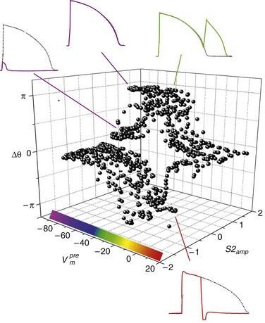
 ). The response was quantified with a cardiac phase variable, θ = arctan[Vm (t + td) − Vm*, Vm (t) − Vm*], where t is time, td = 3 ms, and Vm* = −55 mV (threshold). Regenerative depolarization is characterized by Δθ ≈ +π, and regenerative repolarization by Δθ ≈ −π.81
Cable Phenomena (1D)
 is the length constant, τm = rm cm is the membrane time constant, ri is intracellular axial resistance, and re is extracellular axial resistance (lowercase parameters represent quantities per unit length).
 3) to sustain nonlinear propagation.15
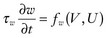 provides the classic FitzHugh-Nagumo equation.12,20 The addition of a slow variable (U) allows a separation of the problem into different time scales, with the result that c = c(U), which allows a quantitative analysis of conduction velocity (CV) restitution. Just as with APD, CV in cardiac tissue is a function of the previous DI and tends to decrease monotonically as DI decreases (and recovery, U, increases), and there is a minimum DI for propagation at a finite CV. CV is highest for fully recovered (resting or quiescent) tissue (Urest) and decreases as U increases until it reaches a critical stall value (Ucrit), that is, propagation occurs for recovery values U < Ucrit, where Ucrit is defined as
Sheet Phenomena (2D)
 . These equations have been confirmed in clever experiments by Cabo et al, in which conduction speed and block through narrow isthmuses in sheets of cardiac tissue were studied; Rcrit was estimated to be ≈1 mm.30 Thus the 2D equivalent of liminal length is that a circle greater than radius Rcrit must be excited to generate a propagating wave because of the effect of wave front curvature; thus the “liminal area” for 2D propagation is
  .
.
![]()
Stay updated, free articles. Join our Telegram channel

Full access? Get Clinical Tree


Thoracic Key
Fastest Thoracic Insight Engine