The noninvasive echocardiographic evaluation of ventricular performance is an essential tool in the clinician’s assessment and management of children and adults with congenital heart disease. As noninvasive methods have continued to evolve, the importance of global and regional ventricular function has become better appreciated. Alterations in both ventricular geometry and loading conditions are the hallmarks of congenital heart disease and can often make the quantitative assessment of ventricular function challenging. This chapter will discuss traditional echocardiographic techniques in the evaluation of ventricular function in patients with congenital heart disease. Newer modalities for functional assessment, including three-dimensional echocardiography, strain and strain rate imaging, and cardiac magnetic resonance imaging, will be covered in greater detail in subsequent chapters in this text.
ECHOCARDIOGRAPHIC ASSESSMENT OF GLOBAL SYSTOLIC VENTRICULAR FUNCTION
Left Ventricular Shortening Fraction
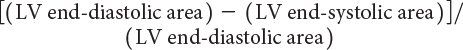
One-dimensional wall motion analysis, or M-mode echocardiography, has traditionally been one of the most commonly used methods to measure the extent of LV shortening. Shortening fraction represents the change in LV short-axis diameter that occurs during systole:

where LVEDD represents LV end-diastolic dimension and LVESD represents LV end-systolic dimension (Fig. 3.1). Normal values for shortening fraction range between 28% and 44%. The short-axis view at the mid-papillary level is the echocardiographic view most frequently used to make these measurements. Similar to shortening fraction, fractional area change can also be measured in this orientation by determining the change in LV area that occurs during the cardiac cycle:
Normal values have been reported to be greater than 36% for fractional area change in adults. LV fractional shortening and fractional area change have been reported to be independent of changes in heart rate and age but are significantly affected by changes in ventricular preload and afterload.
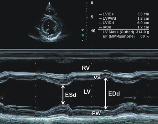
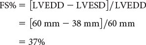
Figure 3.1. Parasternal short-axis image at level of papillary muscles of left ventricle with M-mode measurement of left ventricular shortening.
M-mode–derived shortening fraction (FS%) of left ventricle:
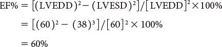
Left ventricular ejection fraction (EF%) can be obtained as follows:
(From Oh JK, Seward JB, Tajik AJ. The echo manual. 3rd ed. [Figure 7-1, p. 110]. Philadelphia, Pa: Lippincott Williams & Wilkins, 2006.)
Left Ventricular Ejection Fraction
LV ejection fraction (LVEF) is the most commonly measured parameter of ventricular function. Global estimation LVEF is often determined in a qualitative fashion; however, using transthoracic or transesophageal echocardiography, two-dimensional echocardiography allows quantitative measurement of LVEF by assessing changes in ventricular volume during the cardiac cycle. The geometric model most commonly used to measure LVEF is the modified Simpson’s biplane method (Fig. 3.2). By using orthogonal apical four-chamber and two-chamber views of the left ventricle, this geometric model calculates LV end-diastolic (LVEDV) and LV end-systolic volume (LVESV) by summing equal sequential slices of LV area from each of these scan planes. LVEF can then be calculated as:
LVEF(%) = [LVEDV – LVESV]/LVEDV × 100
Normal values for LVEF range between 56% and 78%. Similar to shortening fraction, LVEF has been shown to be dependent on changes in ventricular loading conditions.
Accurate calculation of LV volume can occasionally be challenging due to foreshortening of the LV cavity. To circumvent this limitation, the area-length method to derive LVEF can also be used (Fig. 3.3). One of the more commonly used methods, termed the “bullet” method, uses the short-axis area of the left ventricle and the long-axis major LV length (from the apical four-chamber view):

Determination of ventricular volume and EF by this method has been shown to correlate well with invasively measured parameters of ventricular function.
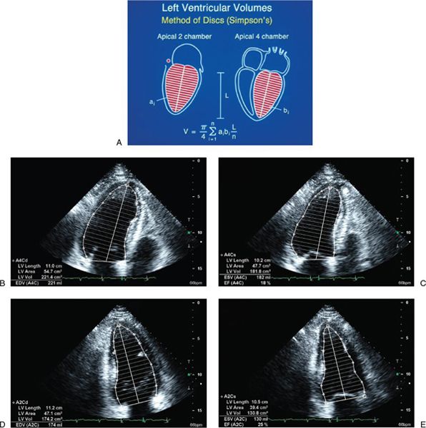
Figure 3.2. Simpson’s biplane methodology to calculate left ventricular (LV) ejection fraction. A: Apical four-chamber and two-chamber views are used to calculate LV volume. LV ejection fraction is assessed from apical four-chamber (B and C) and two-chamber (D and E) views. (A, Adapted from Shiller NB, et al. American Society of Echocardiography Committee on Standards, Subcommittee on Quantitation of Two-dimensional Echocardiograms. Recommendations for quantitation of the left ventricle by two-dimensional echocardiography. J Am Soc Echocardiogr. 1989;2:358–367. B–E, From Oh JK, Seward JB, Tajik AI. The echo manual. 3rd ed. [Figure 7-10, p. 115]. Philadelphia, Pa: Lippincott Williams & Wilkins, 2006.)
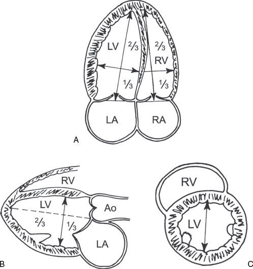
Figure 3.3. Left ventricular (LV) dimensions. A: Mea-surement of the major long-axis and minor short-axis dimension of the left ventricle from the apical four-chamber view. B: Similar measurements of the LV long-axis and short-axis dimensions can be obtained from the parasternal long-axis view. C: LV short axis measured in the parasternal short-axis view. (Adapted from Shiller NB, et al. American Society of Echocardiography Committee on Standards, Subcommittee on Quantitation of Two-dimensional Echocardiograms. Recommendations for quantitation of the left ventricle by two-dimensional echocardiography. J Am Soc Echocardiogr. 1989;2:358–367.)
New echocardiographic technology and advancements in image processing have allowed improved acquisition of ventricular volume. Studies have validated the ability of three-dimensional echocardiography to obtain accurate and reproducible estimates of LV and right ventricular (RV) volumes and EF. While this imaging modality has historically been limited by the time-consuming reconstruction of acquired images, the introduction of real-time three-dimensional imaging has significantly enhanced the quantitative assessment of ventricular volume and function.
Automated border detection (ABD) is another imaging technology that uses acoustic quantification to differentiate the myocardium from the blood pool and thereby allows enhanced visualization of the endocardial border. End-diastolic and end-systolic LV area can be continuously displayed with this modality, enabling determination of ventricular volume, fractional area change, and even pressure-volume or pressure-area loops. Excellent correlation of ABD with other noninvasive and invasive measurements of ventricular function has been reported in some adult studies, but data are lacking in patients with congenital heart disease with altered ventricular geometry.
Left Ventricular Mass
LV mass can be calculated using several echocardiographic methodologies. The unifying principle behind these various measurements is to subtract the volume of the LV cavity from the volume encompassed by the LV epicardium—leaving a “shell” of myocardial muscle volume that can be converted to LV mass by factoring in the specific gravity of myocardium. Devereux and colleagues (1986) have described an M-mode formula to derive LV mass using the short-axis LV dimension as follows:

where 1.04 is the specific gravity of myocardium, LVID is the LV internal dimension, PWT is the posterior wall thickness, IVST is the interventricular septal wall thickness, and 0.8 is a correction factor. Two-dimensional echocardiographic and, more recently, three-dimensional echocardiographic methodologies have been shown to be superior to M-mode–derived measures of LV mass. The two most common two-dimensional approaches include the area-length and the truncated ellipsoid methods. Both of these methodologies use a short-axis view of the left ventricle at the papillary muscle level and an apical four-chamber or two-chamber view to measure the LV long-axis length. LV mass is calculated using LV dimensions and wall thicknesses (measured in centimeters) at end diastole (Fig. 3.4). Normal values for both pediatric and adult cohorts have been published using the area-length or truncated ellipsoid methods.
VELOCITY OF CIRCUMFERENTIAL FIBER SHORTENING AND THE STRESS-VELOCITY INDEX
The rate of LV fiber shortening can be noninvasively assessed by M-mode echocardiography. This measurement, termed the mean velocity of circumferential fiber shortening (Vcf), is normalized for LVEDD and can be obtained from the following equation:

where LVET represents LV ejection time. Reported normal values for mean Vcf are 1.5 ± 0.04 circumferences (circ)/s for neonates and 1.3 ± 0.03 circ/s for children between 2 and 10 years of age. This index assesses not only the degree of fractional shortening but also the rate at which this shortening occurs. To normalize Vcf for variation in heart rate, LVET is divided by the square root of the RR interval to derive a rate-corrected mean velocity of circumferential fiber shortening (Vcfc). Normal Vcfc has been reported to be 1.28 ± 0.22 and 1.08 ± 0.14 circ/s in neonates and children, respectively. Because Vcfc values are corrected for heart rate, a significant decrease in Vcfc between neonates and children has been attributed to increased systemic afterload with advancing age. Vcf is sensitive to changes in contractility and afterload but relatively insensitive to changes in preload. Similar to fractional shortening, this parameter relies on the elliptical shape of the left ventricle and is invalid with altered LV geometry.
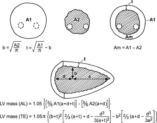
Figure 3.4. Calculation of left ventricular (LV) mass. Calculation of LV mass by the area-length method and truncated ellipsoid method (see text). (Adapted from Shiller NB, et al. American Society of Echocardiography Committee on Standards, Subcommittee on Quantitation of Two-dimensional Echocardiograms. Recommendations for quantitation of the left ventricle by two-dimensional echocardiography. J Am Soc Echocardiogr. 1989;2:358–367.)
Because the majority of ejection phase indices, including shortening fraction, EF, and Vcfc, are dependent on the underlying loading state of the left ventricle, measures of wall tension, namely circumferential and meridional end-systolic wall stress, have been proposed to assess myocardial performance in a relatively load-independent fashion. Colan and colleagues (1984) have previously described a stress-velocity index that is an inverse linear relationship between Vcfc and end-systolic wall stress (Fig. 3.5). This stress-velocity index is independent of preload, is normalized for heart rate, and incorporates afterload, resulting in a noninvasive measure of LV contractility that is independent of ventricular loading conditions. This index can therefore differentiate states of increased ventricular afterload from decreased myocardial contractility. While the stress-velocity index is appealing, the clinical application of this index has been limited by its cumbersome acquisition and its time-consuming off-line. This index is also limited in patients with altered ventricular geometry and wall thickness, features that are hallmarks of congenital heart disease.
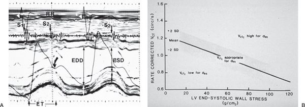
Figure 3.5. Stress-velocity index for assessment of left ventricular (LV) systolic function. A: Parameters used to calculate the stress-velocity index. Note the simultaneous phonocardiogram (identifying the first (S1) and second (S2) heart sounds), ECG, carotid pulse tracing (arrow), and M-mode echocardiogram. Parameters measured include LV end-diastolic (EDD) and end-systolic (ESD) dimensions and LV ejection time (ET). B: Graphic representation of the relationship between the mean rate-corrected velocity of circumferential LV fiber shortening (Vcfc) and the LV end-systolic wall stress (œ es). To normalize Vcf for variation in heart rate, it is divided by the square root of the RR interval to derive a rate-corrected mean velocity of circumferential LV fiber shortening (Vcfc). Values above the upper limit of the mean relationship imply an increased inotropic state, whereas values below the mean imply depressed contractility. (From Colan SD, Borow KM, Neumann A. Left ventricular end-systolic wall stress-velocity of fiber shortening relation: a load independent index of myocardial contractility, J Am Coll Cardiol. 1984;4:715–724.)
Doppler Parameters of Left Ventricular Systolic Function
Echocardiographic evaluation of systolic dysfunction has primarily relied on one-dimensional measures of LV shortening or two-dimensional measures of LV volume change that are often difficult to assess in patients with distorted ventricular geometry. Doppler measures of global ventricular function have been reported to be a potentially more reproducible and sensitive measure of ventricular function.
Left Ventricular dP/dt
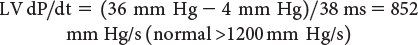
Doppler echocardiography can be used in the quantitative evaluation of LV systolic function. If mitral regurgitation (MR) is present, the peak and mean rate of change in LV systolic pressure (dP/dt) can be derived from the ascending portion of the continuous-wave MR Doppler signal. This rate of change of ventricular pressure is determined during the isovolumic phase of the cardiac cycle before opening of the aortic valve. Using the simplified Bernoulli equation, two velocity points along the MR Doppler envelope are selected from which a corresponding LV pressure change can be derived (Fig. 3.6). This change in LV pressure can then be divided by the change in time between the two Doppler velocities to derive the LV dP/dt. Normal values for mean dP/dt have been reported to be greater than 1200 mm Hg/s for the left ventricle. While more time-consuming to perform, peak dP/dt correlates more accurately with invasive cardiac catheterization measurements. To ascertain peak LV dP/dt noninvasively, the MR signal is digitized to obtain the first derivative of the pressure gradient curve from which peak positive and peak negative LV dP/dt as well as the time constant of relaxation (Tau) can be calculated. While reflective of myocardial contractility, LV dP/dt is significantly affected by changes in preload and afterload.
Myocardial Performance Index (Tei Index)
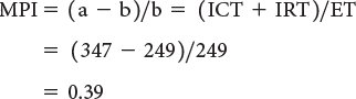
The myocardial performance index (MPI) is a Doppler-derived quantitative measure of global ventricular function that incorporates both systolic and diastolic time intervals. The MPI is defined as the sum of isovolumic contraction time (ICT) and isovolumic relaxation time (IRT) divided by ejection time (ET): MPI = (ICT + IRT)/ET (Fig. 3.7). The components of this index are measured from routine pulsed-wave Doppler signals at the atrioventricular (AV) valve and ventricular outflow tract of either the left or right ventricle. To derive the sum of ICT and IRT, the Doppler-derived ejection time for either ventricle is subtracted from the Doppler interval between cessation and onset of the respective AV valve inflow signal (from the end of the Doppler A wave to the beginning of the Doppier E wave of the next cardiac cycle).
Alternatively, tissue Doppler has been used to measure the MPI. While appealing because of the simultaneous measurement of these time intervals, care needs to be taken because published values for this tissue Doppler technique differ from the pulsed-wave Doppler-derived MPI. Increasing values of the MPI correlate with increasing degrees of global ventricular dysfunction.
Both adult and pediatric studies have established normal values for the MPI. In adults, normal LV and RV MPI values are 0.39 ± 0.05 and 0.28 ± 0.04, respectively. In children, similar values for the LV and RV are reported to be 0.35 ± 0.03 and 0.32 ± 0.03, respectively. The MPI has been shown to be a sensitive predictor of outcome in adult and pediatric patients with acquired and congenital heart disease. Because the MPI incorporates measures of both systolic and diastolic performance, this index may be a more sensitive early measure of ventricular dysfunction in the absence of other overt changes in isolated systolic or diastolic echocardiographic indices. In addition, because the MPI is a Doppler-derived index, it has been reported to be easily applied to the assessment of both LV and RV function as well as complex ventricular geometries found in patients with congenital heart disease. The MPI, however, does have significant limitations. It is significantly affected by changes in loading conditions and has a paradoxical change with high filling pressure or severe semilunar valve regurgitation (“pseudo-normalization”). In addition, the combined nature of this index fails to readily discriminate between abnormalities of systolic or diastolic performance.
ECHOCARDIOGRAPHIC ASSESSMENT OF REGIONAL SYSTOLIC VENTRICULAR FUNCTION
Two-Dimensional Imaging
Both transthoracic and transesophageal echocardiography are ideally suited to evaluate regional wall motion abnormalities. These wall motion abnormalities are characterized by reduced systolic thickening and decreased inward endocardial excursion. Echocardiographic assessment of regional systolic function is best facilitated in the LV short-axis view at the level of the papillary muscles. In the American Society of Echocardiography’s 17-segment model, the left ventricle is divided into six myocardial segments at this level: anterior, anteroseptal, anterolateral, inferolateral, inferior, and inferoseptal (Fig. 3.8). Qualitative visual assessment of wall thickening is graded as normal, hypokinetic (reduced systolic thickening), akinetic (absent systolic thickening), or dyskinetic (paradoxical thinning). Additional views are needed to evaluate all myocardial segments.
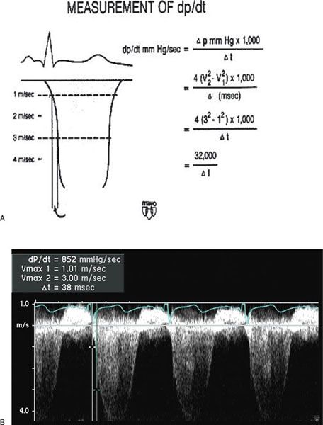
Figure 3.6. Measurement of dP/dt (A) and calculation of left ventricular (LV) dP/dt from the mitral regurgitation jet (B). This still frame demonstrates the Doppler velocity curve of the mitral regurgitation jet obtained during transesophageal echocardiography in a child with dilated cardiomyopathy and severe LV dysfunction. Using the modified Bernoulli equation, the LV dP/dt is the change in LV pressure measured from 1.0 m/s to 3.0 m/s divided by the change in time between these two LV pressure points:
(A, Used with permission from Mayo Clinic.)
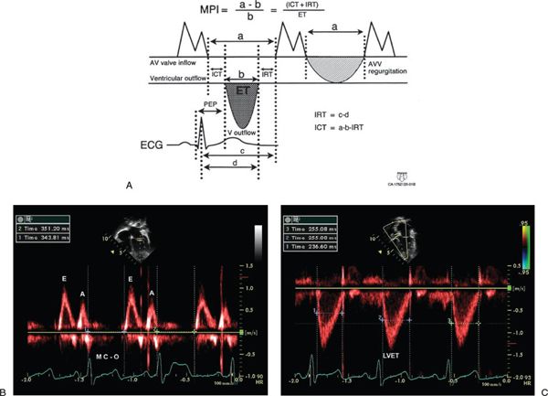
Figure 3.7. Myocardial performance index (MPI) for assessment of left ventricular (LV) global function. A: MPI represents the ratio of isovolumic contraction time (ICT) and isovolumic relaxation time (IRT) to ventricular ejection time (ET): MPI = (ICT + IRT)/ET. B: Pulsed-wave Doppler interrogation in the apical four-chamber view at the level of the mitral valve leaflets. The duration of ICT + IRT is measured from the cessation of mitral valve inflow to the onset of AV valve inflow of the next cardiac cycle (interval a). C: Pulsed-wave Doppler interrogation within the LV outflow tract in the apical five-chamber view. Ventricular ejection time is measured from the onset to cessation of LV ejection (interval b).
(A, From Eidem BW, et al. Nongeometric quantitative assessment of right and left ventricular function: myocardial performance index in normal children and patients with Ebstein anomaly. J Am Soc Echocardiogr. 1998;11:849–856.)
Tissue Doppler Imaging and Strain Rate Imaging
Quantitative assessment of regional systolic LV function, as detailed earlier, has centered on the evaluation of segmental endocardial excursion and LV wall thickening. These semiquantitative methods often fail to discriminate between active and passive myocardial motion. Newer echocardiographic modalities, including tissue Doppler imaging and strain rate imaging, offer a potentially more quantitative and accurate approach to the assessment of regional myocardial contraction and relaxation.
Tissue Doppler echocardiography is a more recent addition to the armamentarium of the echocardiographer. By incorporating a high pass filter, tissue Doppler allows the display and quantitation of the low-velocity high-amplitude Doppler shifts present within the myocardium as opposed to the higher-velocity lower-amplitude Doppler signals more commonly measured within the blood pool (Fig. 3.9). Tissue Doppler is less load-dependent than corresponding Doppler velocities from the blood pool and has systolic and diastolic components. These velocities are heterogenous depending on ventricular wall and position.
Measurement of myocardial wall velocities by TDI has been shown to be a promising modality for assessment of longitudinal systolic performance. Studies have demonstrated significant changes in mitral annular systolic TDI velocities in adult patients with LV dysfunction and elevated LV filling pressures.
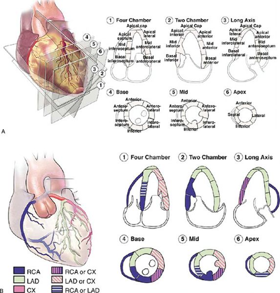
Figure 3.8. Seventeen segment model for analysis of left ventricular wall motion proposed by the American Society of Echocardiography. A: Apical (four-, three-, and two-chamber) and parasternal short-axis views demonstrate the 16 myocardial segments + apical cap. B: Typical coronary artery distribution pattern to these myocardial segments. Note: Coronary arterial supply is variable and may differ from the distribution pattern demonstrated. (From Lang RM, Bierig M, Devereux RB, et al. Recommendations for chamber quantification: a report from the American Society of Echocardiography’s Guidelines and Standards Committee and the Chamber Quantification Writing Group, developed in conjunction with the European Association of Echocardiography, a branch of the European Society of Cardiology. J Am Soc Echocardiogr. 2005;18:1440–1463. Used with permission.)
Tissue Doppler velocities, however, cannot differentiate between active contraction and passive motion, which is a major limitation when assessing regional myocardial function. Regional strain rate corresponds to the rate of regional myocardial deformation and can be calculated from the spatial gradient in myocardial velocity between two neighboring points within the myocardium. Regional strain represents the amount of deformation (expressed as a percentage) or the fractional change in length caused by an applied force and is calculated by integrating the strain rate curve over time during the cardiac cycle. Strain measures the total amount of deformation in either the radial or longitudinal direction, while strain rate calculates the velocity of shortening (Fig. 3.10). These two measurements reflect different aspects of myocardial function and therefore provide complementary information. In contrast to tissue Doppler velocities, these newer indices of myocardial deformation are not influenced by global heart motion or tethering of adjacent segments and therefore are better indices of true regional myocardial function.
ECHOCARDIOGRAPHIC ASSESSMENT OF DIASTOLIC VENTRICULAR FUNCTION
Doppler echocardiography has historically been an essential noninvasive tool in the quantitative assessment of LV diastolic function. Abnormalities of ventricular compliance and relaxation can be demonstrated by characteristic changes in mitral inflow and pulmonary venous Doppler patterns. The addition of newer methodologies, including tissue Doppler echocardiography and flow propagation velocities, enhance the ability of echocardiography to define and quantitate these adverse changes in diastolic performance. Because diastolic dysfunction often precedes systolic dysfunction, careful assessment of diastolic function is mandatory in the noninvasive characterization and serial evaluation of patients with congenital heart disease.

Figure 3.9. A. Normal mitral annular (A), septal annular (B), and tricuspid annular (C) pulsed-wave longitudinal tissue Doppler velocities. Note the normal characteristic pattern of a larger early diastolic velocity (E wave) compared with late diastolic velocity (A= wave). The S wave is the systolic wave. B: Impact of increasing age on tissue Doppler velocities. C: Impact of increasing left ventricular end-diastolic dimension on tissue Doppler velocities. (From Eidem BW, et al. Clinical impact of altered left ventricular loading conditions on Doppler tissue imaging velocities: a study in congenital heart disease. J Am Soc Echocardiogr. 2005;18:830–838.)
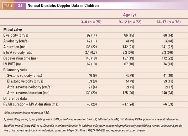
Noninvasive evaluation of diastolic function in normal infants and children is influenced by a variety of factors, including age, heart rate, and the respiratory cycle. Reference values detailing both mitral and pulmonary venous Doppler velocities in a large cohort of normal children have been established (Table 3-1). Similar to many echocardiographic parameters, these Doppler velocities are also significantly affected by loading conditions, making determination of diastolic dysfunction by using these parameters alone very challenging in patients with congenital heart disease.
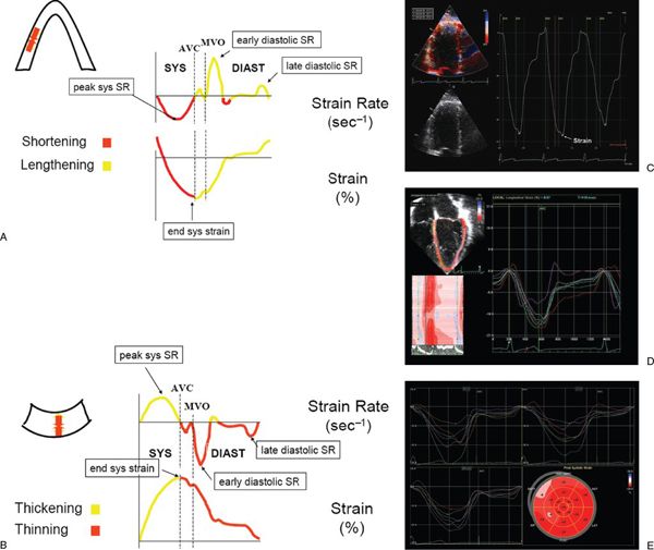
Figure 3.10. Schematic representation of longitudinal (A) and radial (B) strain and strain rate imaging. In the longitudinal direction, strain represents myocardial shortening (systole) and lengthening (diastole), whereas strain rate represents the rate at which shortening or lengthening occurs. Similarly, radial strain represents myocardial thickening (systole) and thinning (diastole), whereas strain rate represents the rate at which thickening or thinning occurs. AVC, aortic valve closure; MVO, mitral valve opening; sys, systolic; diast, diastolic. C: Normal Doppler-based strain acquired in an apical four-chamber orientation at the basal septum. D: Two-dimensional strain obtained in an apical four-chamber view in a normal child. Note the multiple colored curves that represent the various strain patterns in each myocardial segment. E: Two-dimensional strain in a patient with hypertrophic cardiomyopathy. Strain is determined from the apical four-, three-, and two-chamber views. Bull’s eye diagram (bottom right) demonstrates strain in each myocardial segment. Note the decreased strain in the anterior septal, inferior, and septal wall segments. (A and B, used with permission from Luc Mertens, MD.)
Evaluation of Diastolic Ventricular Function—Technical Considerations
A complete Doppler assessment of a ventricle’s diastolic performance must include analysis of the flow signals across the AV valve and within the proximal central venous system (either pulmonary veins for the left ventricle or systemic veins for the right ventricle). Inaccurate assessment will result from attempts to draw conclusions from only one or the other of these flow signals. It is also critically important to obtain these flow signals appropriately or all subsequent conclusions drawn from them will be erroneous. The ultrasound instrument should be set at the lowest frequency and with the smallest sample volume (for pulsed Doppler) possible. This will maximize axial and lateral flow velocity resolution. Low-velocity filtering is used to eliminate tissue motion artifacts. These filters need to be set lower (200 to 600 Hertz) for pulsed-wave interrogation than for continuous-wave Doppler studies (800 to 1200 Hertz). For all signals, the Doppler beam must be aligned as close to parallel as possible with the interrogated flow. Color flow Doppler is extremely useful in achieving optimal alignment.
For AV valve evaluation, the pulsed-wave sample volume is positioned between the tips of the open valve leaflets (Fig. 3.11). This will place the sample volume “below” the anatomic AV valve annulus, at a point within the proximal ventricular inflow tract. In many patients, the apical four-chamber view may not the best position to record AV valve signals. In fact, for the mitral valve, the best alignment is often achieved from the apical long-axis (“two-chamber”) view. This is because normal mitral flow is directed somewhat laterally and posteriorly to the cardiac apex. This flow direction becomes even more pronounced in the dilated heart. Tricuspid inflow signals are often best recorded from a parasternal transducer position. Medial rotation and inferior angulation from the long-axis image will produce a “tricuspid inflow” view that can be used to sample this valve.
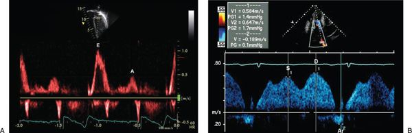
Figure 3.11. Normal mitral inflow (A) and pulmonary venous inflow Doppler (B). E, early diastolic wave; A, atrial filling wave; S, systolic venous wave; D, diastolic venous wave; Ar, atrial reversal wave.
Recordings of central venous flow signals must be made within the vein, not at the junction of the vein and the receiving atrium or vena cava. In adults, it is generally recommended that the sample volume be at least 1 cm “upstream” from the venous orifice. In children, shorter distances must be accepted due to their smaller size, but the sample volume must be placed within the body of the vein to accurately record the flows, especially reversal flows.
The mitral valve inflow signal (Fig. 3.11) is divided into early (E wave) and atrial (A wave) components at the point where the mid-diastolic flow velocity curve changes from a negative to a positive slope (the E-at-A velocity). If no change in slope occurs or if the E-at-A velocity occurs at a velocity greater than one-half of the peak E velocity, then the signal should be considered fused. Deceleration time and total A wave duration should not be measured from fused signals. Mitral A wave duration includes the interval from the E-at-A velocity to cessation of forward flow.
Similarly, division of the pulmonary vein forward flow signal (Fig. 3.11) is made at the point where the flow velocity curve changes slope. Systolic flows occur before and diastolic flows occur after the slope change. Pulmonary vein atrial reversal (PVAR) duration is measured from the onset to cessation of reversed flow occurring after the P wave on the simultaneously recorded, single-lead surface electrocardiogram (ECG). These measurements can be made in the same manner for flow signals recorded at the tricuspid valve and in the systemic (usually hepatic) veins.
Stay updated, free articles. Join our Telegram channel

Full access? Get Clinical Tree


