THREE-DIMENSIONAL ECHOCARDIOGRAPHY IN FUNCTIONAL ASSESSMENT

Assessment of ventricular volumes and ejection fraction is important in patients with congenital and acquired heart disease. Despite intrinsic limitations, ejection fraction still is the most commonly used parameter for ventricular performance. Measurement of ventricular volumes is important in patients with different cardiac conditions such as aortic or pulmonary valve regurgitation. Two-dimensional (2D) echocardiography has been traditionally used for assessing LV and RV volumes and ejection fraction. For the LV, the two most commonly used methods are the biplane Simpson’s method of disks and the area-length method. Both methods depend on geometrical assumptions and use an ellipsoid LV model. In patients with eccentric LV remodelling and LV dilatation, the ventricle becomes more spherical and the LV shape may also be more variable in congenital heart defects. Two-dimensional volumetric assessment of the RV is even more complicated due to its complex geometrical shape, which is difficult to capture in a simplified mathematical formula. The availability of three-dimensional imaging overcomes some of the limitations of the 2D techniques and, especially for assessment of LV volumes and ejection fraction, 3D technology with automated postprocessing, is becoming the technique of choice. The development of 3D matrix probes and automated border detection techniques have made 3D techniques more easily accessible for clinical use.

From Reconstruction Techniques to Real-Time Three-Dimensional Imaging

The development of 3D echocardiography imaging was a logical but challenging technological development. Already in the 1970s initial attempts were made to record and display images of the heart in three dimensions. At that time, off-line 3D reconstruction from serial ECG-gated acquisitions of multiple 2D planes was performed either by freehand scanning or a mechanically driven transducer that sequentially recorded images at predefined intervals. With freehand scanning, a series of images were obtained by manually tilting the transducer along a fixed plane, and a spatial locator attached to the transducer translated the 3D spatial location into a Cartesian coordinate system. The main disadvantage of this approach was the relative bulk of the spatial locator device, which made transducer manipulation difficult, and extensive postprocessing was required. Freehand scanning used a mechanical transducer for obtaining serial images at predefined intervals either in parallel planes or by pivoting around a fixed axis in a rotational, fan-like manner. Because the intervals and angles between the 2D images were defined, a 3D coordinate system could be derived from the 2D images in which the volume was more uniformly sampled. This approach, although accurate, required long acquisition and postprocessing times. The quality of 3D reconstruction from 2D images depended on a number of factors, including the intrinsic quality of the 2D data set, the number of 2D images used, the ability to limit motion artifacts, adequate ECG, and respiratory gating. It also relied on the assumption that all planes are acquired at the same phase of the respiratory cycle to ensure identical shape and position of the heart within the chest. Finally, the need to shorten the acquisition times in order to minimize motion artifacts, made image quality often suboptimal. Later, the use of multiplane probes emerged as a readily available method to obtain rotational images at predefined angles around a fixed axis.

An important milestone in the history of 3D echocardiography was reached in the early 2000s, with the development of fully sampled matrix array transducers. These transducers allow the creation of real-time 3D images. The need for tedious multiplane acquisition was eliminated. This novel approach is based on real-time volumetric 3D imaging. This advance in 3D imaging saved computer interpolation of cross-sectional images and thus could avoid spatial motion artifacts. Real-time 3D echocardiography uses transducers containing arrays of piezoelectric elements capable of acquiring pyramidal data sets. It is now possible to depict cardiac motion at a sufficient frame rate during a single breath hold without the need for off-line reconstruction, thus eliminating motion artifacts known to adversely affect the reconstruction methodologies.

Technical Aspects

Real-time 3D echocardiography uses matrix array transducers with elements arranged in a grid fashion, typically containing more than 3000 imaging elements transmitting at 2 to 4 MHz for transthoracic imaging. The availability of a higher frequency probe (7 MHz) made it possible to obtain real-time 3D images with improved spatial resolution in younger children and infants. The matrix probes are computationally demanding, and to reduce the size of the connecting cable, miniaturized circuit boards are incorporated into the transducer, allowing partial beam forming within the transducer. More recent developments resulted in a smaller transducer footprint, improved side lobe suppression, and harmonic capabilities. These probes can acquire data sets at 360-degree focusing and have electronic steering for volumetric acquisition at satisfactory spatial resolution (voxel size, 0.5 3 0.5 3 0.6 mm) with acceptable temporal resolution (30 to 40 frames/s).

Real-time 3D systems generally have two methods for data acquisition: real-time, also called live 3D imaging, and electrocardiographically gated multi-beat 3D imaging. Real-time imaging refers to the acquisition of multiple pyramidal data sets over a single heartbeat. Real-time 3D data can be acquired in three modes: narrow-angle; zoom, magnified; and wide-angle. Although these modes overcome the limitations imposed by rhythm disturbances or breathing motion, the data sets are acquired at lower spatial and temporal resolution. The real-time narrow mode displays a pyramid of approximately 60 3 30 degrees that permits visualization of a single, relatively small structure like the aortic valve, in any one imaging plane with good spatial resolution. The zoom mode displays a magnified, wide pyramid of 30 3 30 degrees (Video 4.1). The wide-angle shows a pyramidal data set of approximately 90 3 90 degrees. Wide-angle data sets provide larger pyramidal scans at the cost of lower spatial resolution compared with narrow-angle acquisition.

Multi-beat 3D imaging provides images of higher temporal resolution through the acquisition of four to eight narrow volumes of data over several heartbeats that are subsequently stitched together to create a single volumetric data set (Video 4.2). Multi-beat imaging allows the acquisition of the largest sector possible at a reasonable temporal resolution of 30–40 frames per second. The full volume allows entire visualization of large structures such as the LV, RV, and valves. The full volume can be rotated to orient structures in face views (Fig. 4.1). These data sets can also be cropped or transected in any plane in order to better visualize specific anatomic structures (Fig. 4.2). Multi-beat volumetric imaging is inherently prone to artifacts created by irregular heart rhythm or motion (breathing). To minimize reconstruction artifacts, data should be acquired during breath holding if possible.

Recognizing and avoiding potential artifacts is critical for an accurate interpretation of 3D data. Artifacts are mainly related to respiratory motion in patients unable to hold their breath, like young children. Motion artifacts may result in stitching artifacts when the four sub-volumes are merged. ECG gating can be challenging in patients with arrhythmias, including normal sinus arrhythmia. Importantly, in real-time 3D echocardiography, image quality is closely related to the intrinsic 2D images used to produce the 3D data set. When the 2D images are poor then the 3D images are generally even poorer and should not be acquired. The use of optimal gain settings is essential for accurate diagnosis. Low gain settings can artificially fade certain structures that will not be viewable during postprocessing. In contrast, excess gain leads to a decreased spatial resolution and loss in the 3D perspective. It is generally recommended to use higher gain settings during acquisition with adjustment of the gain settings during postprocessing.

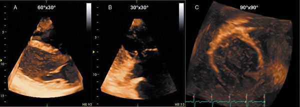
Figure 4.1. Three different three-dimensional data acquisition modes. A: Real-time narrow-angle imaging mode. B: Zoom mode, which allows visualization of small structures such as a coaptation abnormality of the tricuspid valve. C: Wide-angle full-volume data set; this data set is acquired over four to seven heartbeats.

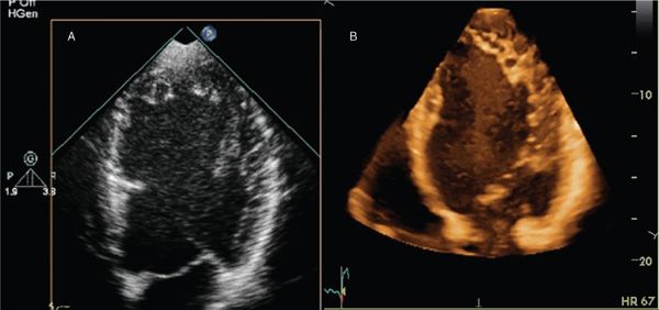
Figure 4.2. A two-dimensional (2D) (A) and full-volume three-dimensional (3D) (B) data sets cropped to view cardiac structures of interest in a patient with left ventricular noncompaction. Compared with the 2D image, the 3D image shows depth information at the cost of lower spatial resolution.

In 3D imaging there is an important trade-off between spatial and temporal resolution (volume rates). To improve spatial resolution, an increase in the number of scan lines per volume is required; this, however, takes longer to acquire and reduces temporal resolution. Imaging volumes should be made as small as possible to increase temporal resolution while maintaining spatial resolution.

Imaging Protocols

A complete 3D echocardiogram should include assessment of ventricular morphology, volumes and function, valve morphology, and hemodynamic data. In general, 3D echocardiography is performed as a complement to a 2D study. Although a 3D full-volume acquisition mode can accommodate almost the entire heart with existing technology, the decrease in spatial and temporal resolution that would result from enlarging the volume to acquire the entire heart from a single acoustic window makes this impractical. Therefore, 3D data sets are acquired from multiple transducer positions. For example, focused 3D imaging for LV volume quantification typically can be performed with an apical four-chamber wide-angle acquisition complementing standard 2D imaging (Fig. 4.3 and Video 4.3). An advantage of 3D echocardiography compared with 2D echocardiography is that quantitative analysis does not rely on the ability of the operator to acquire images positioned properly in certain standard views relative to cardiac anatomy. Unlike 2D echocardiography, in which standard views are described based on the plane through which they pass, 3D echocardiography is inherently volumetric. As such, full-volume data sets of the beating heart, which can be rotated and sliced in any plane, allow the reader both an external view of the heart and multiple internal views with the use of cropping (Video 4.4). Essential components of a full 3D echocardiogram for assessment of ventricular function include wide-angle acquisition of a parasternal long-axis view, an apical 4-chamber view, and a subcostal view including color interrogation of all valves. Visualization, description, and analysis of images are generally performed in three orthogonal planes: (a) the sagittal plane, which corresponds to a vertical long-axis view of the heart; (b) the coronal plane, which corresponds to a four-chamber view; and (c) the transverse plane, which corresponds to a short-axis view. Each plane can be viewed from two sides, representing opposite perspectives. For example, the transverse plane can be viewed from the apex or the base of the heart. The choice of narrow- or wide-angle acquisition depends on the structure to be visualized. For smaller structures, such as valves, a narrow-angle acquisition is more appropriate. For imaging the ventricles, it is best to use a wide-angle acquisition in the apical window so that the entire volume of the ventricles can be covered. Acquisition is followed by off-line analysis with dedicated 3D software. This requires cropping and tilting of the data set. Because a data set comprises the entire ventricular volume, multiple slices can be obtained from base to apex to evaluate wall motion. An advantage of 3D over 2D imaging is the possibility of manipulating the plane to align the true long and short axes of the left ventricle, avoiding foreshortening and oblique imaging planes.

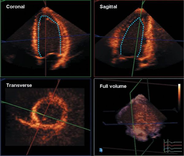
Figure 4.3. A full-volume data set (bottom right) cropped into coronal, sagittal, and transverse planes. Such data sets are used to delineate endocardial and epicardial borders and calculate ventricular volumes, mass, and ejection fraction.

Clinical Applications

Assessment of LV Volumes and Ejection Fraction

Accurate and reproducible quantitative assessment of LV size and mass, as well as regional and global LV function, are important components of an echocardiogram. They are pivotal for diagnosis, treatment, and prognosis of patients with different heart diseases. Multiple methods for measuring LV size and function have been developed for both M-mode and 2D echocardiography. The relative inaccuracy of these one-dimensional (1D) and 2D approaches has been attributed to the need for geometric modeling of the ventricle, assuming the left ventricle is an ellipsoid. The lack of information on one dimension, the “missing dimension,” has been considered the main source of the wide inter-measurement variability of the echocardiographic estimates of LV size and function. This is particularly true in children with congenital heart disease whose ventricles have distorted morphology and do not follow geometric models that are generally used. An advantage of 3D echocardiography over 2D imaging is that it provides full-volumetric data sets, so there is no need for geometric modeling. Several studies comparing 3D echocardiography with magnetic resonance imaging (MRI) as a gold standard have shown that the quantification of LV volumes and function with 3D echocardiography is highly feasible, reproducible, and accurate when compared with LV volumes measured by MRI (Fig. 4.4).

Visualization of the endocardial surface can be challenging, especially in the apical lateral and anterior myocardial segments. This can be compensated for by tilting the transducer, which improves endocardial visualization at the expense of generating foreshortened views of the left ventricle, resulting in a potential source of error when calculating LV volumes. Despite the high correlation with MRI, studies have shown 3D echocardiography slightly underestimates LV volumes. This is believed to be due to the inability of 3D echocardiography to identify the myocardial borders as accurately as MRI. In addition, the lower temporal resolution of 3D echocardiography may lead to the inability to capture the real end-systolic frame. This can lead to inaccurate end-systolic volume measurements.

In the past, 3D echocardiographic quantification of LV volumes and function required tedious manual delineation of subendocardial borders in multiple planes. Today, most vendors offer a nearly fully automated frame-by-frame detection of the endocardial surface. Typically this process involves segmentation of the 3D data set into two or three equiangular 2D longitudinal planes. This requires indicating a few anatomical landmarks such as the septal, lateral, anterior, and inferior mitral annuli at end diastole and end systole. If necessary, manual corrections can be performed after automated analysis. The software calculates LV volumes in each frame, endocardial wall motion, and ejection fraction (with the use of no geometrical assumptions) by detecting the endocardial blood interface. Models of the left ventricle and data from normal LVs, however, guide border detection methods. The data sets can be displayed as a volume-rendered or surface-rendered image (Figs. 4.5 and 4.6 and Videos 4.5 and 4.6).

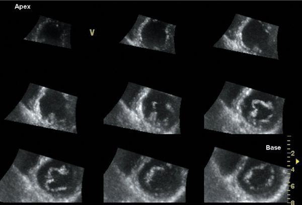
Figure 4.4. Multislice short-axis display of a full-volume data set. Cropping and rotation in any desired plane allows the operator to render the true short-axis views covering the entire left ventricle from base to apex. This display is useful to evaluate wall motion abnormalities because it allows direct comparison among different myocardial segments.

Three-dimensional echocardiography also allows calculation of LV mass. Two-dimensional echocardiography derives LV mass from measurements of myocardial wall thickness at one site and uses geometrical formulas. This leads to inaccuracies, especially when wall thickness is inhomogeneous, as occurs in asymmetric hypertrophic cardiomyopathy. Three-dimensional echocardiography seems to overcome this limitation because it allows calculation of wall thickness in all myocardial segments. Three-dimensional echocardiographic measurement of LV mass requires the delineation of endocardial as well as epicardial borders. While M-mode overestimates LV mass and 2D echocardiography underestimates LV mass, 3D echocardiographic measurements have been shown to correlate highly with MRI mass calculation.

The current analysis programs also allow calculation of regional myocardial function based on the 3D data sets. Changes in regional volumes can be calculated and regional volumetric curves can be displayed for each sub-volume. This allows quantification of regional myocardial function. Speckle-tracking technology can also be applied to the volumetric data sets to calculate 3D strain. A clinically useful byproduct of the 3D quantification of regional LV wall motion is the ability to quantify the temporal aspects of regional systolic wall thickening. The standard deviation of regional time to peak ejection times (interval between the R wave and peak systolic endocardial motion) has been used as an index of myocardial synchrony (Figs. 4.7 and 4.8 and Videos 4.7 and 4.8). This index can also be used to select candidates and to guide resynchronization therapy. A reduction in acquisition time makes 3D echocardiography particularly suited to stress echocardiography in which there is a narrow temporal window to acquire images at peak stress. The downside is the lower frame rates at higher heart rates. The benefit of this methodology in pediatric heart disease awaits further studies.

RV Volumes and Ejection Fraction

An accurate evaluation of RV size and function is of great importance in patients with congenital heart disease. However, imaging the RV is challenging due to its complex shape, its anterior position in the chest, and its thin walls with deep trabeculations. Mainly because of the more complete morphology of the RV walls, cardiac MRI is considered the clinical reference technique for measuring RV volumes and ejection fraction. Even when using cardiac MRI, standardization in image acquisition and postprocessing is essential for reducing interobserver variability. In younger children, cardiac MRI requires general anesthesia and is not readily available for serial measurements.

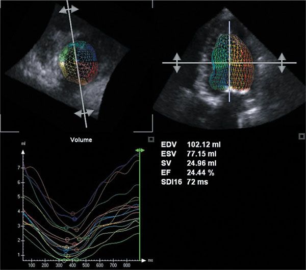
Figure 4.5. Calculation of left ventricular end-diastolic and end-systolic volumes, stroke volume, and ejection fraction in a 4-year-old with aortic stenosis and heart failure. Note that ventricular volumes are increased and ejection fraction is reduced. Also, significant heterogeneity in regional volumes indicating differences in regional myocardial function is seen (bottom left).

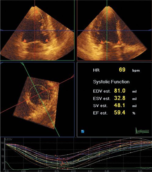
Figure 4.6. Analysis of left ventricular global and regional function, as well as global and regional volume curves with three-dimensional echocardiography. The endocardial border is semiautomatically traced after manual indication of the mitral annuli and apex in two orthogonal views (triangles) at end diastole and end systole.

In theory, 3D echocardiography could be a good alternative to cardiac MRI for the assessment of RV shape and function. This requires a specific acquisition of RV volumes to capture the different RV walls in the volumetric data set. Specific postprocessing software is available for analyzing RV volumes and ejection fraction. This still is a semi-automated method requiring more extensive postprocessing compared to LV volumetric analysis (Fig. 4.9). Another limitation is that good quality data sets are often difficult to obtain, as visualization of the entire right ventricle from a single data set is often not possible. It is not uncommon that a part of the RV outflow tract cannot be included in the data set. This is particularly problematic for the more dilated RV, limiting the feasibility of this method, especially in adult patients (Video 4.9).

Different studies have tried to validate this methodology in different patient groups and compared the volumetric 3D RV data with measurements obtained by cardiac MRI. While certain studies report reasonable accuracy, the majority of the studies report a systematic underestimation of RV volumes using the echocardiographic methods, especially when the RV is more significantly dilated. Some groups have tried to subsegment the RV volumes into inlet, apical body, and RV outlet.

An alternative method for quantifying RV volumes uses 2D images positioned in 3D space using a magnetic tracker attached to the probe. On the 2D images, anatomic landmarks are identified and these landmarks, localized in 3D space, are used for reconstructing the RV volumes based on a database of RV shapes. This method has the advantage of being less dependent on the acquisition of full-volumetric 3D data sets and, as based on 2D images, is more often successful in obtaining reliable RV data. It has also been shown to be highly reproducible, and the RV volumes obtained using this method correlate well with the volumes obtained by cardiac MRI. The disadvantage of this method is that it requires the use of a magnetic tracking device and specific software and the online access to the database of RV shapes. This limits the accessibility of the methodology.

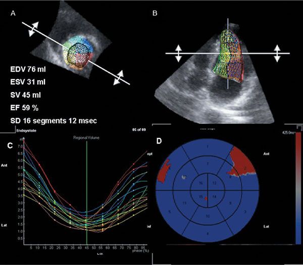
Figure 4.7. Assessment of left ventricular synchrony in a normal subject. A and B: Ventricular volumes, ejection fraction, and synchronicity index calculated as standard deviation in time from R wave to minimal regional volume in 16 myocardial segments. Note small variation among myocardial segments. C: Regional myocardial volume curves throughout the cardiac cycle. D: Bull’s eye representation of the same data. Note homogeneous activation pattern with slightly more delayed activation of the basal septal and basal lateral myocardial segments.

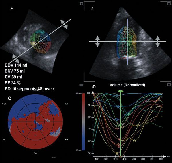
Figure 4.8. Assessment of left ventricular synchrony in a child with dilated cardiomyopathy. Note enlarged left ventricular volumes with reduced ejection fraction and large standard deviation of time from R wave to minimal regional volume; this indicated dyssynchrony (A and B). C: Bull’s eye representation demonstrating earlier activation of the interventricular septum and inferior wall with delayed activation of the basal anterior and lateral myocardial segments. D: Curves with marked dispersion of time to minimal regional volume.

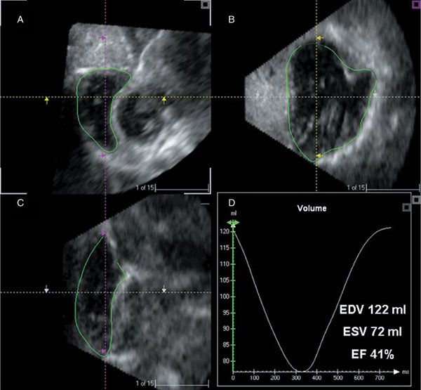
Figure 4.9. Right ventricular analysis program displaying three-dimensional ultrasound images in sagittal (A), four-chamber (B), and coronal (C) views at end diastole. By manual tracing of endocardial borders at end diastole and end systole in all planes, one can calculate right ventricular volumes and ejection fraction (D).

Assessment Volumes and Ejection Fraction in the Single Ventricle

Assessment of single ventricular function remains a clinical challenge and in clinical practice is still largely based on subjective assessment. Having a more quantitative method available for clinical follow-up would certainly be useful. Full-volumetric acquisition with postprocessing using either LV or RV software depending on the morphology of the dominant ventricle could theoretically be used. There has been some validation of this methodology in various types of single ventricles. This earlier work was based on a method of disks, which requires extensive postprocessing and is no longer readily commercially available. Data on the more automated methods for assessing RV function are scarce. There are intrinsic limitations to the application of the 3D methodology to single ventricles. The most important one is that it can be very difficult or impossible to get the entire single ventricle in the volumetric data set. A second problem is that in case there is a smaller second ventricle also contributing to cardiac output, the analysis can become even more complicated. Finally, the identification of the different walls of the single ventricle can be difficult, limiting the feasibility and reliability of the method.

Additional potential applications of real-time 3D echocardiography in pediatric heart disease that are beyond the scope of this chapter include (a) measurement of left atrial volumes, which is considered to reflect chronic diastolic function and left atrial pressure; (b) quantification of ventricular volumes in the fetal heart; (c) visualization of valve morphology, calculation of valve area, and quantification of regurgitant volumes; (d) guidance of transcatheter interventions such as atrial septal defect device closure, electrophysiologic studies, and intraoperative monitoring; and (e) description of complex congenital heart lesions.

Future Directions

Future advances in transducer and computer technology should focus on higher frequency transducers for smaller children with a smaller footprint. Also, better temporal and spatial resolution of the 3D images would bring additional diagnostic benefit. Better 3D representation of the images and data sets through the development of 3D screens, holographic projection, and 3D printing techniques would allow better understanding of 3D anatomy. Finally, combining 3D echocardiography with MRI or computed tomography (CT) images may yield fusion data sets with unsurpassed anatomic, functional, and physiologic information.

TISSUE-DOPPLER IMAGING FOR THE EVALUATION OF MYOCARDIAL FUNCTION

Most of the traditional echocardiographic techniques used to assess ventricular function look at either dimensional changes caused by ventricular contraction or study the effect of cardiac events utilizing blood pool Doppler. All this indirectly reflects what is happening within the cardiac wall during the cardiac cycle. A different approach is to look directly into the myocardium and measure regional function by quantifying myocardial properties like velocities and deformation throughout the cardiac cycle. Tissue-Doppler imaging (TDI) was the first technique developed for studying myocardial motion. By adjusting machine filter settings, tissue velocities in the myocardium can be measured (Fig. 4.10). The initial description did not raise a lot of clinical interest; but when experimental data confirmed that, in normal myocardium, changes in segmental systolic velocities were linked to changes in regional contractility, there was a renewed interest in the measurement. Several clinical studies subsequently investigated the value of measuring regional myocardial velocities in various diseases such as ischemic heart disease, aortic insufficiency, and hypertrophic cardiomyopathy. In ischemic heart disease, it was demonstrated that tissue velocities changed very quickly (within 5 s) after the induction of myocardial ischemia in a pig model and was one of the earliest changes observed. Also for pediatric and congenital heart disease, this technique was considered to be potentially useful, as it directly looks into the myocardial walls and is independent of ventricular geometry. Myocardial velocities can be measured using pulsed-wave (PW) Doppler: a sample volume of 4–8 mm can be placed within the myocardium while trying to align the ultrasound beam as parallel as possible to the direction of motion studied by the technique (Fig. 4.11). Alignment is important, as all Doppler-based techniques are angle-dependent. The velocity waveform represents the instantaneous velocity in the region of interest throughout the cardiac cycle. PW Doppler has a very high temporal resolution (250–300 frames/s). The spatial resolution is limited because the sample volume does not track the translational motion of the underlying myocardial segment as the segment moves through the sample volume. A normal pulsed-wave tissue-Doppler imaging trace obtained in the basal part of the interventricular septum is shown in Figure 4.11. Different peaks can be noted. During the isovolumic contraction period, there is a short-lived peak corresponding to the myocardial shape change that occurs during this period. When the fibers contract against closed valves, there is a change from a more spherical to an ellipsoid shape. During the ejection phase there is a systolic waveform that can be measured that corresponds to the base-to-apex motion of the myocardium during systole. Normally this waveform peaks during the first one third of the cardiac cycle corresponding to the maximal force development early in systole. During the isovolumic relaxation period, another short-living velocity peak can often be recorded. In diastole two peaks are present: an early diastolic peak corresponding to early filling and a late diastolic peak occurring during atrial contraction. These velocities represent the opposite motion of the atrioventricular valve from the apex toward the base in diastole. As with all Doppler techniques, by convention, motion toward the transducer is represented as positive waves and motion away from the transducer as negative waves. In current clinical practice PW Doppler is used to quantify longitudinal myocardial motion by measuring mitral and tricuspid annular velocities. For the mitral annulus this can be measured in the septum or in the LV lateral wall. Peak septal velocities are lower compared to the LV lateral wall velocities. Peak tricuspid annular velocities are higher compared to mitral annular velocities.

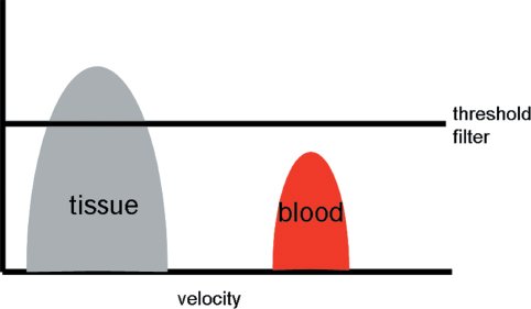
Figure 4.10. Principles of tissue-Doppler. The tissue signals have higher amplitude but lower velocity while the blood pool signals have lower amplitude but higher velocity. By adjusting the threshold filter settings the tissue-Doppler velocity tracings can be detected.

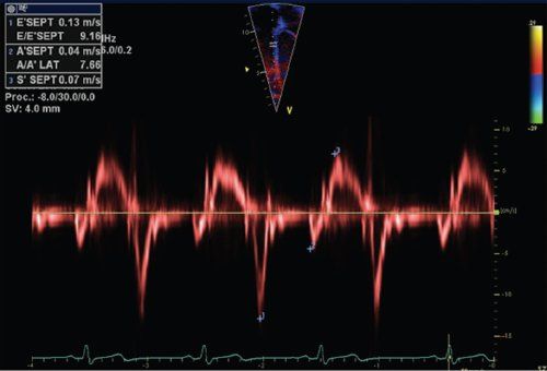
Figure 4.11. Pulsed Doppler tracing obtained in the basal part of the interventricular septum. The pulsed-wave Doppler sample volume is placed in the basal part of the interventricular septum just below the mitral valve annulus. Different peak velocities can be measured: systolic peak velocity during ejection (S’), early diastolic peak velocity (E’) and diastolic peak velocity during atrial contraction (A’).

Tissue-Doppler velocities can also be measured using color tissue-Doppler imaging (CTDI). It was introduced in the early 1990s based on the same principles as color Doppler blood pool imaging. Using auto-correlation techniques, regional mean velocities instead of peak tissue velocities are measured. The difference in measurement technique explains why CTDI-derived myocardial velocities are on average 15–20% lower compared to PW Doppler myocardial velocities. The CTDI images are displayed as color images using the same color-coding used for blood pool color Doppler imaging with myocardial velocities toward the transducer displayed in red, and velocities away from the transducer in blue (Fig. 4.12). The color-coded tissue-Doppler information can be stored digitally and, by using postprocessing software, any velocity curve can be displayed at any point within the color Doppler information, allowing measurements at different sites in the myocardium during the same cardiac cycle. When narrowing the sector and optimizing the machine settings, high-frame rates to .250 fps can be obtained. This is important as certain myocardial mechanical events are short-lived and require high-frame rates. As with any Doppler technique, alignment with the direction of myocardial motion is important. Compared with PW TDI, CTDI has the advantage that velocities in different myocardial segments and walls can be recorded simultaneously during the same cardiac cycle. This allows comparing the regional wall motion and timing of cardiac events between different myocardial segments within the same cardiac cycle. This can be useful in the evaluation of the synchronicity of the contraction pattern in different myocardial wall segments and can also be used for calculating myocardial velocity gradients within a myocardial wall. This is the basis of TDI-based strain and strain rate imaging, which has largely been replaced by speckle-tracking echocardiography in clinical practice, but has been an important research technique.

Current Clinical Applications of Tissue Velocities

Multiple experimental and clinical studies have been performed to characterize the myocardial velocity profile in normal subjects. Systolic myocardial velocities have been used to look at systolic function, and in adults, measurement of peak early diastolic velocity (E’) has become a key component in the assessment of diastolic function, both for grading diastolic dysfunction as well as in the assessment of LV filling pressures. Velocities are vectors expressed relative to a coordinate system. In the cardiac coordinate system, motion is described relative to the longitudinal, radial, and circumferential direction (Fig. 4.13). This differs from an intrinsic coordinate system that ideally should be based on actual fiber orientation. In the epicardium, myofibers are predominantly obliquely and more longitudinally oriented in a left-handed helix. In the LV, the fiber orientation changes from epicardium to endocardium—from oblique to circumferential in the midwall into a right-handed obliquely oriented helix in the endocardium. The underlying fiber orientation influences the velocities measured in a certain direction or axis. In the longitudinal direction, systolic and diastolic myocardial velocities are higher at the base of the heart and decrease toward the apex, which remains almost stationary. Due to a predominant longitudinal motion in the RV, the tricuspid annular tissue-Doppler velocities are higher than the LV longitudinal velocities. When analyzing radial myocardial function, myocardial velocities are higher at the endocardium than at the epicardium. For these reasons, a gradient in myocardial velocities exists between the base and the apex (in the longitudinal direction), and between the endo- and epicardium. This velocity gradient can be measured and represents myocardial strain rate (the rate of deformation in a certain segment). When integrating the strain rate curve versus time, myocardial strain can be calculated. With the advent of speckle-tracking echocardiography, these techniques have become obsolete in clinical practice.

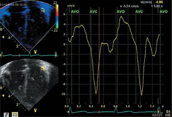
Figure 4.12. Color Doppler myocardial imaging. An apical four–chamber view is obtained with color tissue–Doppler imaging. From the color-velocity data, tissue velocity curves can be extracted and on these traces the same velocity peaks can be identified as on the pulsed-wave traces (S’, E’, and A’). The advantage of color Doppler myocardial imaging is that velocities in different segments can be recorded during the same cardiac cycle. This allows comparing velocities in different segments during the same cardiac cycle.

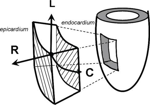
Figure 4.13. The cardiac coordinate system. This is the cardiac coordinate system used as a reference system for tissue-Doppler vector velocities and myocardial deformation imaging. Velocities and deformation are expressed in the longitudinal (L), radial (R), and circumferential (C) direction. Longitudinal velocities are measured from apical views; radial from short-axis or long-axis views; circumferential from short-axis views.

Use of Tissue-Doppler Velocities in Children

Normal values for PW tissue-Doppler velocities in children have been published in different studies. In children, myocardial velocities vary with age, heart rate, and myocardial segment. A study published by Eidem et al. included 325 children from different ages. They showed that pulsed-wave tissue-Doppler velocities are influenced by cardiac growth, especially by left ventricular (LV) end-diastolic dimension and LV mass. Similar findings have been reported during fetal growth with a progressive increase in tissue-Doppler velocities with increase in cardiac size. This indicates that tissue velocities are, to some degree, influenced by ventricular geometry, which has significant implications when applying this methodology to children with congenital heart disease. A possible solution to this problem has been proposed by Roberson et al. who expressed normal TDI velocities as z-scores normalized for BSA. In adult studies, peak tissue-Doppler velocities were initially reported to be relatively load-independent, while later studies could demonstrate the influence of loading conditions (preload and afterload) on peak systolic and early diastolic tissue velocities. A distinction has to be made between acute changes in loading conditions and chronic pressure or volume loading. Cardiac remodeling (eccentric or concentric hypertrophy) associated with chronic loading can result in normalization of loading conditions, which can also result in a normalization of the tissue-Doppler patterns. Acute changes in preload and afterload generally influence peak systolic tissue-Doppler velocities, while velocities may normalize again in chronically adapted ventricles. Eidem et al. studied the effect of different congenital abnormalities on tissue-Doppler velocities in children. In patients with dilated cardiomyopathy, systolic tissue velocities were reduced in the different segments, consistent with a reduced ventricular systolic function in this patient group (Fig. 4.14). In children with ventricular septal defects, basal septal velocities were only very mildly reduced with normal systolic and diastolic peak velocities in the LV basal lateral wall. In contrast, children with aortic valve stenosis had reduced systolic basal velocities that were reduced in both the septum and the lateral wall when compared to velocities in a normal control group. This suggests that longitudinal systolic function is decreased in patients with aortic stenosis. Similar observations were made by Kiraly et al. with decreased systolic and diastolic tissue velocities in the lateral and posterior LV walls with longitudinal velocities more significantly reduced compared to radial velocities in children with aortic stenosis. Weidemann et al. showed that in adult patients with aortic stenosis the degree of reduction in LV longitudinal function is predictive of the degree of myocardial fibrosis as observed during surgery. Data for children are not available, however.

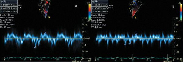
Figure 4.14. Longitudinal systolic tissue velocities in patient with dilated cardiomyopathy. This 8-year-old child was diagnosed with dilated cardiomyopathy with globally reduced LV systolic function. The longitudinal tissue-Doppler velocities as obtained in the LV basal interventricular septum (A) and lateral wall (B) are significantly reduced.

Stay updated, free articles. Join our Telegram channel

Join