FIGURE 7.1. Mass and spring model for tissue mechanics. The ultrasound transmission properties of tissue can be derived by considering the tissue to be assembled from masses (representing tissue density) and springs (representing tissue stiffness). No wave: At rest, with no wave present, the masses are equally distributed in the tissue. Transverse wave: If a transverse wave passes through the tissue, the displacement of the tissues can be seen, like the lateral displacement as a wave passes along a rope. Longitudinal wave: Ultrasound passes through tissue as a longitudinal wave, with regions of tissue compression and regions of tissue decompression. Pressure fluctuation and molecular velocity: The pressure fluctuation and the molecular velocity are in phase; the ratio of pressure fluctuation to molecular velocity is the tissue impedance. The acceleration is 1/4 cycle ahead of the molecular velocity and the displacement is 1/4 cycle delayed.

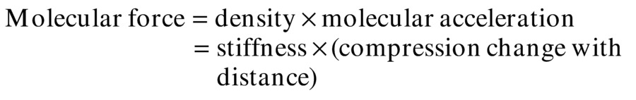
When these equations are applied to molecules in a material, the compression force is set equal to the acceleration force:
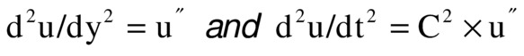
Ultrasound wave mechanics are derived from this equation. If u is the distance of each molecule from its resting position, y is distance along the direction that the wave is traveling, and t is time, the previous equations become

where the second derivatives d2u/dt2 and d2u/dy2 represent tissue acceleration and tissue distortion, respectively. These equations can be solved by assuming that molecular displacement u is dependent on the variable group (y + C × t) having units of centimeters; C has units of centimeters per second (cm/s). The previous derivatives can then be expressed as
and the equation becomes
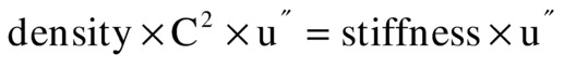
Therefore, for any waveshape of u, the equation is correct if C2 = (stiffness/density). In this equation, C2 is positive, but the value of C can be either positive or negative, and it is the speed of the ultrasound wave.
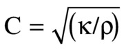
The meaning of C is further understood by looking at Figure 7.2. The wave has different locations at different times. As time advances (from top to bottom), the wave moves from left to right. The line marked “wave speed” shows a place on the wave near a crest where the value (y + C × t) is constant. In Figure 7.2, C is negative; thus, as time increases, y must also increase to keep (y + C × t) constant. The expression (y + C × t) provides the relationship between advancing time and advancing location, which is speed. The wave period T (the time it takes to change from one peak to the next) and the wavelength λ (the distance it takes to change from one peak to the next) are related by C, the wave speed:
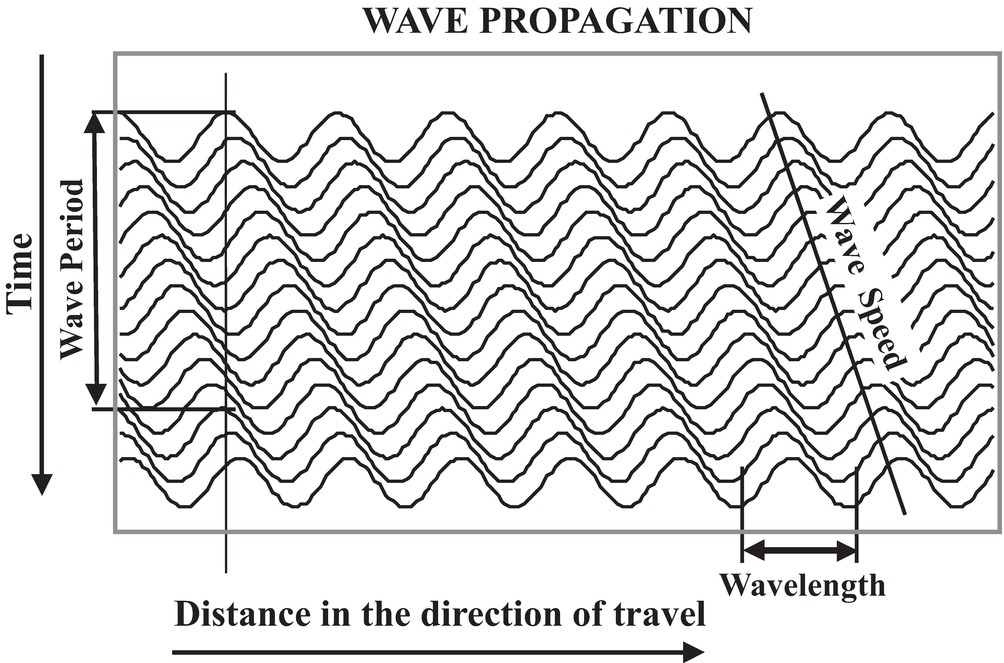
FIGURE 7.2. Wave propagation over time. As a wave travels through a medium, the wave length (λ) and the wave period (T = 1/F) are related by the wave speed (C = λ/T = λ × F). The wave function is dependent on the variable (y − C × t) where y is the distance along the direction of travel and t is time.

Wave period (T) is the inverse of frequency (F), so that
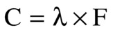
The following equation is also an important relationship to remember for any longitudinal mechanical (sound) wave traveling through a material:
where κ is stiffness and ρ is density. Of course, both stiffness and density depend on temperature; thus, C will vary with temperature.
The speed of sound in typical soft tissue is 1540 m/s or 1.54 mm/μs, whereas the speed of sound in air is 331 m/s. These are determined by the density and stiffness of the materials. Typical sound and ultrasound wavelengths are presented in Table 7.1.
TABLE 7.1 Sound Wavelengths for Different Frequencies
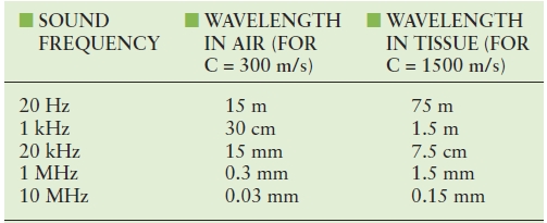
C, wave speed (see text).
Ultrasound Frequencies and Wavelength
Frequency is measured in hertz, which is an expression of cycles of compression and decompression per second. Medical ultrasound frequencies are measured in millions of cycles per second, or megahertz (MHz). Wavelength is related to the spatial resolution of an ultrasound image. Because your ears are about 15 cm apart, you cannot tell where a 20-Hz sound (15-m wavelength in air) is coming from, but you can identify where a 2-kHz sound (15-cm wavelength in air) is coming from. By using 5-MHz ultrasound in tissue (0.3-mm wavelength), it is possible to resolve objects that are a few millimeters apart.
Impedance and Wave Speed
As a sound pulse (or wave) travels through tissue, zones of high pressure and low pressure are created. The high-pressure regions occur where the molecules are squeezed together, and the low-pressure regions occur where the molecules are spread apart. The pressure elevation or depression from atmospheric pressure is called pressure fluctuation (p). Pressure fluctuation is equal to the stiffness (κ) times du/dy. As a sound pulse travels through tissue, the molecules oscillate in the direction of the sound wave. The instantaneous molecular velocity (v) of the oscillating molecules is du/dt, and because u is dependent on (y + C × t), du/dt = C × du/dy. Therefore, v/C = p/κ, or
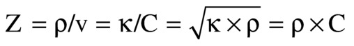
Z is called the acoustic impedance of the tissue. In physical terms, impedance is the ratio between the pressure fluctuation that the tissue feels as a wave passes and the molecular velocity of the molecules as the wave passes. Be sure to avoid confusing the molecular velocity of the molecules (v) with the wave speed (C). The molecular velocity (v) oscillates in the positive and negative directions during ultrasound wave passage at the ultrasound frequency; v is greater when the wave intensity is greater. C is the speed at which the wave passes and does not change with wave intensity, as long as the intensity is low. If the intensity is high, the “linear” model of springs and masses in Figure 7.1 does not hold. The “nonlinear” waves at higher intensities cause harmonics, which are the basis of harmonic imaging (discussed later in this chapter).
It is important to remember that impedance (Z), like wave speed (C), is dependent on the density and the stiffness (1/elasticity) of the tissue. Just as wave speed changes with temperature, impedance changes with temperature because temperature affects both stiffness and density.
Amplitude and Phase
In addition to the wavelength (in units of distance) and period (in units of time), each wave has two other properties: the amplitude and the phase (Fig. 7.3). All of the information in a wave is encoded in the amplitude and phase. Ultrasound B-mode imaging displays the echo amplitude, and Doppler velocity information is acquired from the phase. These two kinds of information are independent: one can change while the other remains constant.
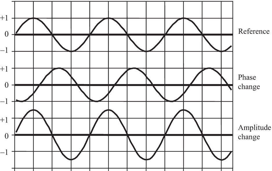
FIGURE 7.3. Wave phase and amplitude. Two parameters define a wave of a particular frequency: the amplitude and the phase. The amplitude of a wave is taken as the peak difference of a parameter from ambient conditions. In ultrasound, the parameter is usually pressure fluctuation from atmospheric pressure, but could be molecular velocity, acceleration, or displacement. Amplitude of the ultrasonic echo is used for B-mode imaging. The phase is the time difference of a wave feature from the same feature on a reference wave. Therefore, phase is always represented as a difference. That difference could be in time or in distance along the propagation direction.
The amplitude of a sound wave can be measured in many different ways, but each method measures properties experienced by the molecules of the material through which the sound is traveling. Each molecule experiences a pressure fluctuation, which is a displacement back and forth along the direction of wave travel associated with a molecular velocity and acceleration. The displacement, velocity, and acceleration are like the displacement, velocity, and acceleration of a swing or a pendulum.
Frequency and phase are closely related. When a 5-MHz Doppler looks at an approaching blood velocity of 75 cm/s, the Doppler echo has a frequency of 5.005 MHz. The frequency is increased by 0.1% or 1/1000 of the transmit frequency. Another way to think of this is that the phase becomes more advanced with every cycle: for every 1000 cycles, the phase has advanced 1 cycle. After the first 10 cycles, the phase has advanced 1/100 of a cycle. Because one cycle is 360 degrees, after 10 cycles, the phase has advanced 3.6 degrees, and after 100 cycles, the phase has advanced 36 degrees. It can be convenient to think about the Doppler shift as a continuing change in phase rather than a frequency shift.
Pressure Fluctuation and Molecular Velocity, Displacement, and Acceleration
Molecular velocity, displacement, acceleration, and pressure are related to ultrasound intensity. These four measured values are ways to look at the mechanical “shaking” that the molecules experience as an ultrasound wave passes through the tissue. First, ultrasound intensity is related to energy:

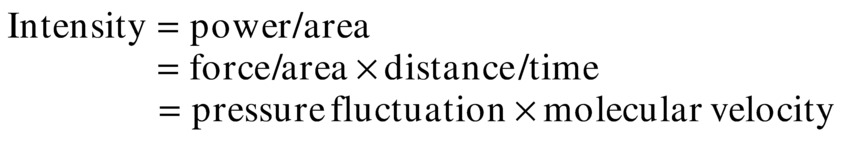
As discussed earlier, the pressure fluctuation is the fluctuation of the pressure in the tissue due to the passing of an ultrasound wave; the molecular velocity is the velocity of molecules in the tissue due to the passing of the ultrasound wave.
As shown previously, in the solution to Newton’s equations, the ratio of tissue pressure fluctuation to molecular velocity fluctuation represents the tissue impedance (Z):

By substitution:
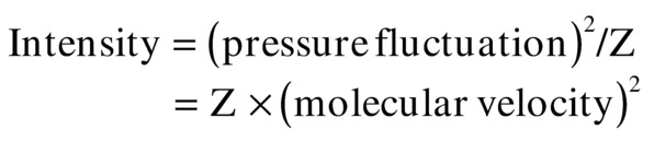
If the ultrasound is continuous wave (CW), the average intensity is the average of the sine wave amplitude squared. That average is half of the squared maximum value:
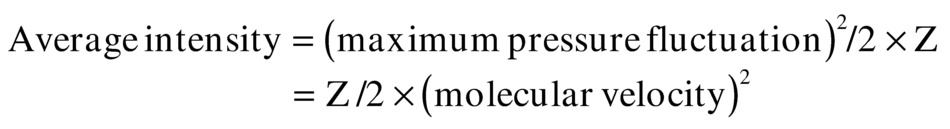
This is also true within an ultrasound pulse. The temporal peak intensity is computed from this same expression.
A graph of the pressure fluctuations versus CW intensity (Fig. 7.4) indicates that a physical problem occurs within the range of diagnostic ultrasound intensities: at temporal peak intensities greater than 320 mW/cm2, the pressure fluctuation becomes greater than 1 atm. Therefore, the minimum pressure theoretically becomes negative. This is impossible according to the physical laws of thermodynamics. Thus, the linear equation for compressibility, which is based on thermodynamics, does not apply for these conditions. The wave becomes nonlinear (Fig. 7.5) and gives rise to harmonics.
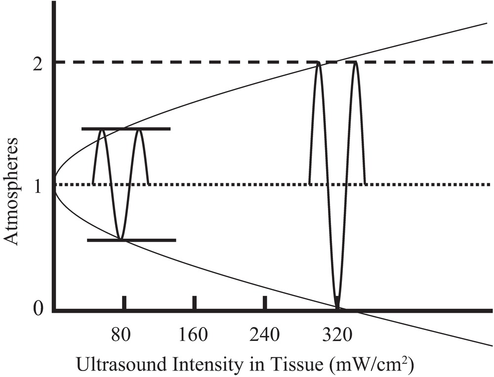
FIGURE 7.4. Tissue pressure fluctuation versus medical ultrasound intensity. Intensity is equal to one-half of the square of the peak pressure fluctuation divided by the tissue impedance. Using the impedance of water, which is near the impedance of human tissues, at an intensity of 320 mW/cm2 (SPTP), the pressure fluctuation equals 1 atm.
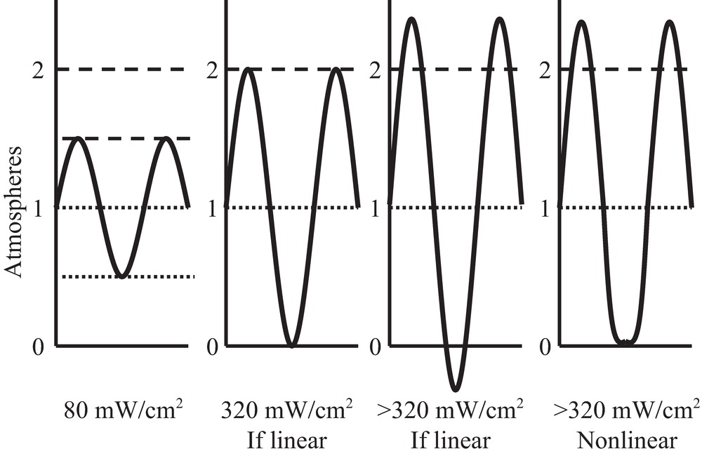
FIGURE 7.5. Ultrasound waveshape changes with nonlinear propagation. As an ultrasound sine wave propagates through tissue, the shape of the wave changes: the peaks increase in height and sharpness, and the valleys become blunted. This effect is greater at higher intensities. This change in shape is due to nonlinear stiffness of the tissue, which causes the wave velocity to be higher when the pressure is at the peaks and the wave velocity to be lower when the minimum pressure is at or below zero.
Nonlinear Mechanics
With nonlinear mechanics, the linear equations presented earlier no longer apply. The relationship between pressure and displacement, which is based on the nature of molecular bonds, does not hold for large fluctuations in pressure.
The nonlinear relationship between compression and force is shown in Figure 7.6. In the central region, stiffness is linear, but when compression becomes too great or too small, the effective stiffness changes. When the wave intensity is very large, during compression, the stiffness is increased, causing an increase in the wave speed and an increase in the wave impedance. Likewise, during decompression, the stiffness is decreased, causing decreases in both the wave “speed” and “impedance.” Speed and impedance are in quotation marks in these cases because their definitions become less useful in these nonlinear conditions than in the linear conditions.
FIGURE 7.6. Nonlinear behavior of tissue stiffness. Near atmospheric pressure, the compressional force is linearly related to the change in dimension of the tissue, but at higher or lower pressures, the force significantly deviates from linear. The addition of an acoustic contrast agent consisting of bubbles expands the tissue and increases the nonlinearity.
Harmonics and Ultrasound Contrast Agents
The flattened valleys and the enhanced peaks of the waveshape in Figure 7.5 (right) can be represented as a combination of sine waves (Fig. 7.7). In this example, a sine wave at the original frequency and a sine wave at two times the original frequency are shown. The wave at the original frequency is called the fundamental; the wave at two times the frequency is called a harmonic. The wave at two times the fundamental frequency is called by different names: it is called the “first harmonic” by some people and the “second harmonic” by others. Both groups agree on the name “first overtone” for that frequency. Harmonics occur at two times, three times, or any integer multiple of the fundamental. Any periodic (repeating) waveshape can be formed from a series of sine wave harmonics of the fundamental by selecting the phase and the amplitude of each harmonic. This is the Fourier theorem and is the basis of the Fourier transform. The lower curve in Figure 7.7 shows the combination of the fundamental and the harmonic.
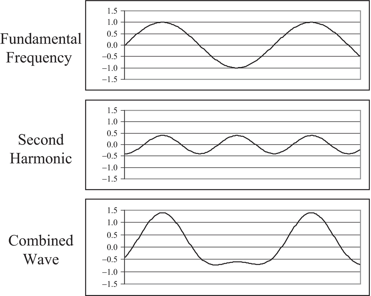
FIGURE 7.7. Harmonic components of nonsinusoidal waves. Any periodic repeating wave can be represented by a series of sine waves starting with the fundamental and adding wave frequencies that are multiples of the fundamental. These waves are harmonics. The first harmonic is the fundamental, the second harmonic has a frequency twice that of the fundamental, and so on. Each harmonic has a unique amplitude and phase that it contributes to the combined wave. Here, 1.5 cycles of the fundamental (top) are added to 3 cycles of the second harmonic (middle) with a phase that causes the peaks to align, producing a wave with blunted minimums and enhanced maximums (bottom). The combined wave is similar to the wave in Figure 7.5 that resulted from nonlinear propagation in tissue.
Harmonics are present in all diagnostic ultrasound echoes. If the transmitted intensity is increased, the intensity of the harmonics increases as more of the power from the fundamental frequency is converted to the harmonics. The attenuation of ultrasound is proportional to frequency; thus, the harmonics are attenuated more rapidly than the fundamental. Some of that attenuation is due to absorption (conversion to heat), so that if the ultrasound intensity is doubled, the amount of ultrasound converted to heat more than doubles because of the conversion to harmonics and the subsequent conversion to heat.
The subject of harmonics has been recognized for decades but was not often discussed until recently, and harmonic displays are relatively recent additions to diagnostic ultrasound instruments. Interest in the display of harmonics is primarily a result of a general desire to improve detection of ultrasound contrast agents. When ultrasound contrast agents were introduced, they were designed to increase the strength of the echo signals in ultrasound images. However, they did not produce the strong echoes on images that were hoped for. This led to the development of methods to display harmonics. The bubbles in ultrasound contrast agents will change the linear portions of the line in Figure 7.6 and cause the generation of harmonics. Thus, displaying harmonic echoes was expected to show contrast agents more prominently. However, tissues without contrast agents also reflect harmonic echoes back to the transducer (Fig. 7.8). In general, tissue harmonic imaging improves the lateral resolution and image contrast.
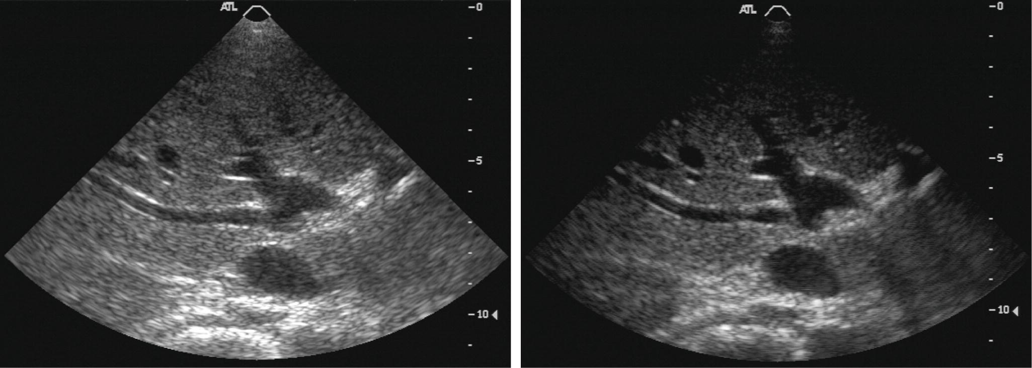
FIGURE 7.8. Harmonic image of liver without contrast agent. In typical medical ultrasound imaging, the SPTP intensities are much higher than 320 mW/cm2, so nonlinear wave propagation and the formation of harmonics are common. An image formed by showing the amplitude of the fundamental frequency echo (left) looks different from an image of the same tissue formed by transmitting a lower frequency and forming an image based on the strength of the second harmonic of the transmitted frequency (right).
To generate a harmonic image using a 3-MHz transducer, it is logical to transmit at 3 MHz and receive at 6 MHz, but this cannot be done because a transducer is not sensitive at even multiples of the frequency. The 3-MHz transducer must have a “damping” material to make it “broadband,” so that it will operate between 1.5 and 4.5 MHz. Then, for harmonic imaging, it is possible to reduce the transmit frequency to 2 MHz and increase the receive frequency to select 4-MHz echoes to generate the harmonic image.
Transmitted Ultrasound
Continuous Wave
CW ultrasound is used for Doppler applications. The instruments are generally inexpensive and often provide nondirectional audible output. However, CW Doppler instruments can provide directional information, and they can also produce spectral waveforms. The transmitted ultrasound is “narrowband” because only one ultrasound frequency is transmitted. Because the transmission is continuous, no information about the depth of the detected flow is available.
Burst and Pulse
The terms pulse and burst have similar meanings. Pulse refers to the shortest burst of ultrasound that can be sent into tissue with the transducer available. Burst refers to an intentionally prolonged transmit oscillation. For most diagnostic imaging applications, the transmitted ultrasound pulse is on for a short period of time (Fig. 7.9), less than a microsecond, and off for 100 μs. For most pulsed Doppler applications, a burst of ultrasound lasting 1 μs is sent into tissue. For transcranial Doppler applications, the transmitted burst may last 15 μs. Long transmit bursts are narrowband, so they define the Doppler frequency with precision and they are resistant to noise. For B-mode imaging, a short (broadband) transmit pulse is used to ensure the best (smallest) depth resolution. This allows the visualization of small structures in the depth direction, like the intima-media thickness.
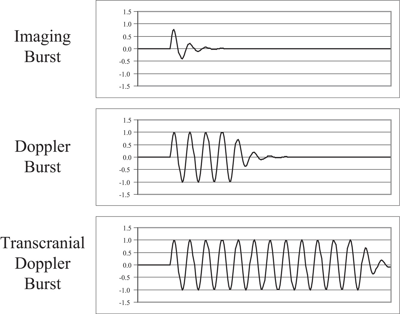
FIGURE 7.9. Burst length of ultrasound pulses. For B-mode imaging, short (broadband) ultrasound bursts are transmitted into tissue (top) to get the best depth resolution. For Doppler, medium-length ultrasound bursts are transmitted into tissue (middle). For transcranial Doppler, in which the echoes are greatly attenuated and the transmitted burst energy must be high while limiting the SPTP intensity, long (narrowband) ultrasound bursts are transmitted into tissue (bottom).
During the “off” period, the receiver is accepting echoes from successively deeper locations. This period lasts between 40 and 400 μs. An ultrasound instrument computes the depth of the echo reflector by measuring the time from the transmit pulse to the echo, assuming an ultrasound speed of 1.54 mm/μs. Echoes from shallow structures (1 cm deep) return soon after the transmit pulse (about 13 μs); echoes from deeper structures (3 cm deep) return later after the transmit pulse (about 40 μs); echoes from the deepest structures (25 cm deep) return latest (about 325 μs) (Table 7.2).
TABLE 7.2 Time Required for an Echo to Return from a Known Depth
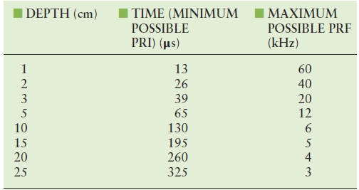
PRF, pulse repetition frequency; PRI, pulse repetition interval.
Duty Factor
The duty factor (DF; or duty cycle) is a measure of the fraction of time that the ultrasound instrument is transmitting. In a CW instrument, the system is always transmitting, and the DF is 1.0, or 100%. In a pulse-echo B-mode ultrasound instrument imaging a maximum depth of 19 cm, the transmit pulse is 1 μs, and the pulse repetition period (PRP; time between pulses) is 250 μs. Thus, the DF is 1/250, or 0.004, or 0.4%. The concept of DF also applies to a home heating system. To heat a home on a cool day, the furnace might be on for 15 minutes out of every hour (DF = 25%), but on a cold day, the furnace might be on for 30 minutes out of every hour (DF = 50%). The DF is an important part of the computation of ultrasound intensities.
Power and Intensity
There is a great deal of confusion in ultrasound physics literature about power and intensity. Here is the reason for the confusion. Power is a measure of energy per time and has units of watts. As an ultrasonic wave passes through tissue, the power is distributed over the cross-sectional area of the ultrasound beam pattern. Power divided by the cross-sectional area is equal to the intensity. The intensity is easily measured with an ultrasound transducer called a hydrophone and determines whether the ultrasound propagation is linear or nonlinear. Intensity is related to pressure fluctuation and is therefore the quantity usually discussed in ultrasound physics. Intensity is dependent on both the ultrasound power in the beam pattern and the cross-sectional area of the beam pattern. Changes in intensity due to changes in cross-sectional area of the beam pattern can easily be confused with changes in intensity due to changes in ultrasound power. It is important to keep the two factors separate.
In tissue, ultrasound power decreases with distance as the wave propagates. The decrease in power is due to attenuation in the tissue. Attenuation has two factors: (1) conversion of the ultrasound power to heat (absorption) and (2) scattering of the ultrasound power in directions other than the direction of the ultrasound beam. The attenuation (both absorption and scattering) of ultrasound in tissue is dependent on the tissue type and the ultrasound frequency.
Measures of Ultrasound Intensity
There are six common measures of ultrasound intensity:
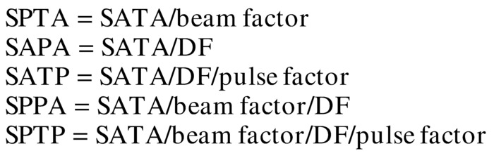
- Spatial average temporal average (SATA)
- Spatial peak temporal average (SPTA)
- Spatial average pulse average (SAPA)
- Spatial peak pulse average (SPPA)
- Spatial average temporal peak (SATP)
- Spatial peak temporal peak (SPTP)
Between 1980 and 1990, the number of measures was changed from four to six, and the naming of the measures changed. The new measures are pulse average values, which were previously called “temporal peak.” Temporal peak now refers to an instantaneous peak value rather than a value averaged over the pulse. Two of the six measures (SATA and SPTA) are used for computing heating effects; the rest are used for considering ultrasonic cavitation and nonlinear effects of ultrasound.
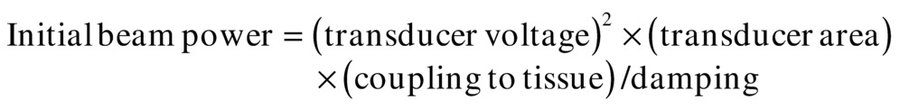
All of these are measures of an ultrasound transmit beam and depend on two factors: (1) the beam power and (2) the beam area. The initial power of the beam is selected by applying the proper voltage to the ultrasound transducer based on the transducer thickness, the damping material on the back of the transducer, the area of the face of the transducer, and the efficiency of coupling to the body tissues under examination:
As the ultrasound pulse proceeds into tissue, the beam power decreases owing to attenuation:

The beam area is dependent on the focal character of the transducer. Intensity is the ratio of beam power to beam area:

The beam power can be expressed as a maximum or as a temporal average.
The most widely accepted method of measuring the ultrasound beam is to begin with a measurement of the total beam power. Beam power is measured by directing the beam onto a submerged weighing pan of a standard balance. When the ultrasound beam strikes the pan, a force appears. The force is equal to

In water, where the speed of sound is 148,000 cm/s, a 1-W temporal average ultrasound beam generates a force equal to the weight of a 1.38-mg mass. This force can be demonstrated by imaging water in a tank. By turning up the gain, particles suspended in the water can be seen. As the transmit power is increased, the suspended particles can be seen on the ultrasound image rushing away from the ultrasound scanhead because of the ultrasound force. By measuring the ultrasound beam with a hydrophone, the beam diameter and area can be determined. From these measurements, the SATA intensity can be determined:

A look at the interrelationships of the six intensity terms listed above can provide a more complete picture of tissue exposure. The intensity measures are related by combinations of four factors: (1) duty factor (Fig. 7.10), (2) beam factor (Fig. 7.11), (3) pulse factor (Fig. 7.12), and (4) image factor (Fig. 7.13). These four factors all have the same range: maximum = 1, minimum = 0. Using a hydrophone and an oscilloscope (which traces the voltage in time that is generated by the hydrophone), the factors shown in Figures 7.10 to 7.13 can be determined. Then, the intensities can be computed:
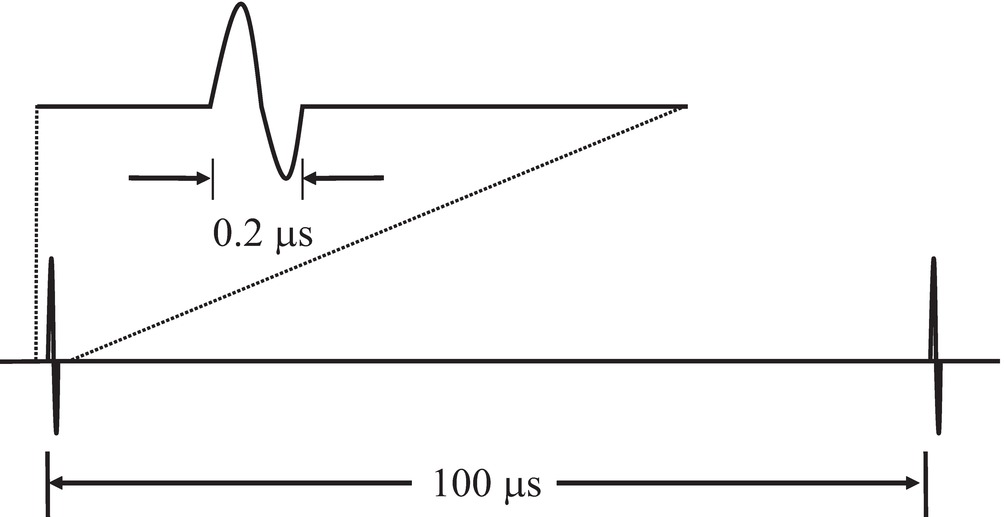
FIGURE 7.10. Duty factor. The duration of an ultrasound transmit burst (top) is short compared with the time interval separating bursts (bottom). The ratio of burst length to interval is called the duty factor.
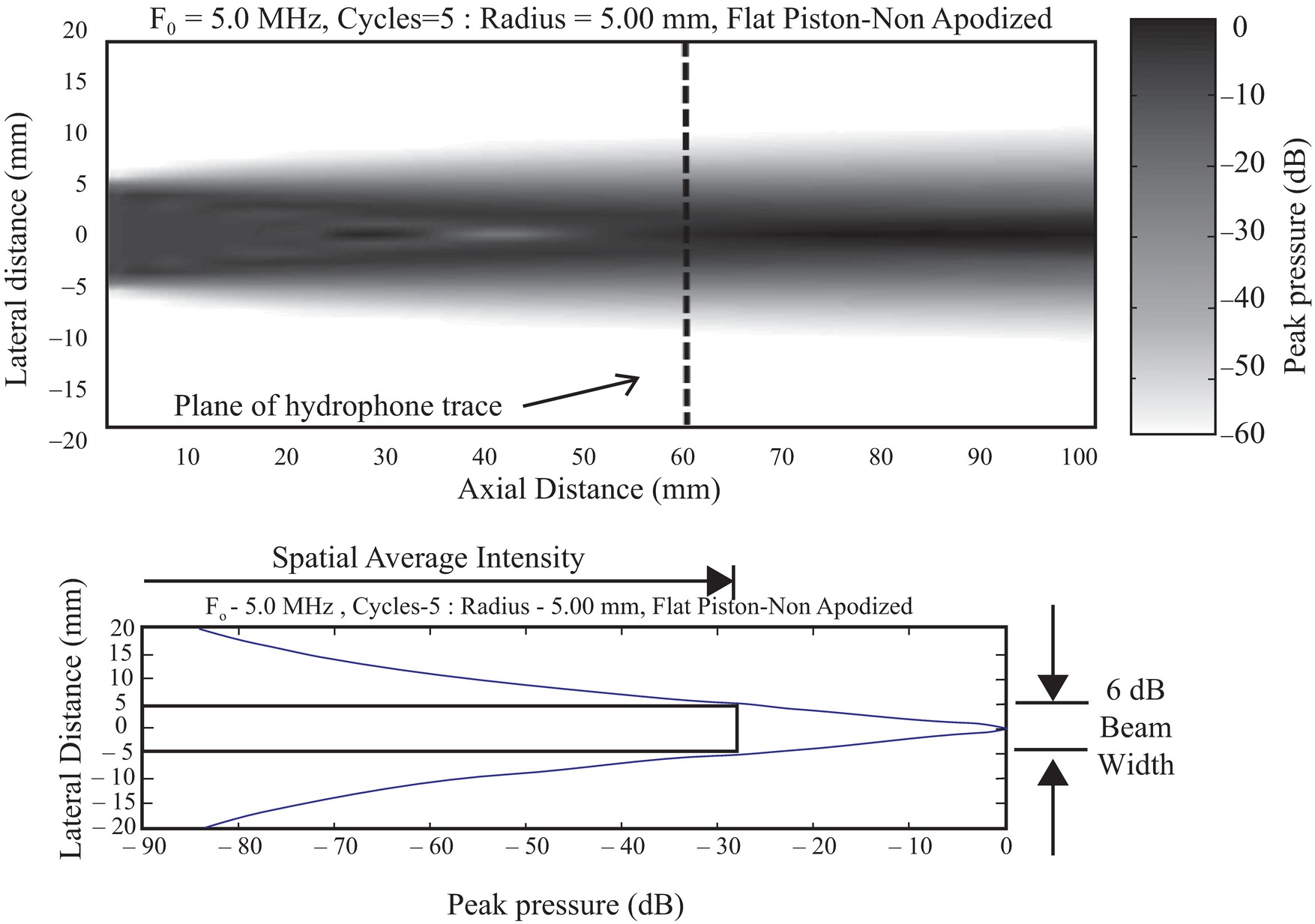
FIGURE 7.11. Beam factor. Top,The beam pattern of a flat circular transducer extends from the face of the transducer into tissue. Near the transducer in the Fresnel zone is a complex area of varying intensity formed by diffraction, which is the constructive and destructive interference of the waves from the transducer face. Far from the transducer in the Fraunhofer zone, the beam pattern becomes much smoother. Bottom,A profile of the maximum pressure fluctuation taken across the beam at the transition zone between the Fresnel and the Fraunhofer zones shows the intensity peak. A box is drawn that shows the width of the central portions of the beam where intensities are at least 25% (>6 dB) of the peak. The spatial average intensity across that beam width is between one-half and one-third of the central peak intensity.
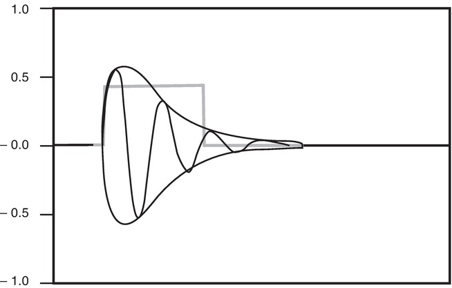
FIGURE 7.12. Pulse factor. The oscillations show the acoustic pressure applied to the tissue, with a gradual onset and decay. During each half-cycle, the energy is proportional to the square of the amplitude, indicated by the envelope of the pulse. The square pulse is a simplified model of the ultrasound burst power showing the temporal average power for the duration of the pulse. The pulse average power is less than the instantaneous temporal peak power of the pulse.

FIGURE 7.13. Image factor. The 2D B-mode image is formed from more than 100 pulse-echo lines. Therefore, the average intensity exposure of tissue on any one line is equal to the exposure computed for repeat exposures if all pulses were delivered along a single line, divided by the number of lines in the image.
Different ultrasound modes have different DFs (Table 7.3). In some examinations, the ultrasound beam is held stationary (A-mode, M-mode, and pulsed Doppler). For 2D imaging, however, the scanhead sweeps the ultrasound beam across a plane of tissue, penetrating each element of tissue only once per image frame for 2D B-mode, and typically eight times per image for 2D color Doppler. Thus, in 2D imaging, the image factor must be included in exposure computations for a voxel (a small volume) of tissue, indicating the number of ultrasound scan lines per image that are acquired from other locations in tissue. This allows an increase in the energy in each transmit burst, because only one ultrasound pulse passes through each voxel of tissue in each frame. The frame rate is usually about 30 images/s; thus, only 30 pulses/s heat each segment of tissue. However, because the bursts have higher energy, they have high peak positive and negative pressures, which thereby increase the chance of cavitation in the tissue.
TABLE 7.3 Transmit Parameters for Ultrasound Examination Methods
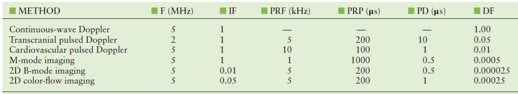
DF, duty factor (dimensionless); F, ultrasound frequency; IF, image factor = 1/number of ultrasound lines in an image (dimensionless); PD, pulse duration = length of transmit pulse or burst (s); PRF, pulse repetition frequency = number of transmitted pulses per second (Hz); PRP, pulse repetition period = 1/PRF (s); 2D, two-dimensional.
Theoretical Intensities versus Actual Intensities
Unknown factors, such as the attenuation of overlying tissue and refractive spreading of the ultrasound beam, make correct theoretical computations of the ultrasound intensities impossible. Experimental investigations of ultrasound intensities must be performed if accurate values are to be known. Unfortunately, properly mimicking the conditions of an examination and then placing a calibrated hydrophone at the location of maximum intensity (a location that is unknown within the depths of tissue) to determine the maximum intensity is either difficult or impossible. Almost any conceivable arrangement is seriously flawed. Thus, we are left with a few general conclusions:
1. The computed intensities and, consequently, the computed heating effects are generally more severe than any actually achieved in the body tissues.
2. Caution demands that ultrasound examinations be limited to minimum transmit powers (and therefore maximum receiver gain settings) consistent with achieving diagnostic data.
3. Caution also demands that ultrasound image acquisition be limited to the shortest possible time and that for demonstrations and discussions, the freeze frame and cine functions on the system be used whenever possible.
4. Examiner training should begin with learning about the proper use of the instrumentation so that the recommendations in conclusions 2 and 3 above can be followed.
Attenuation
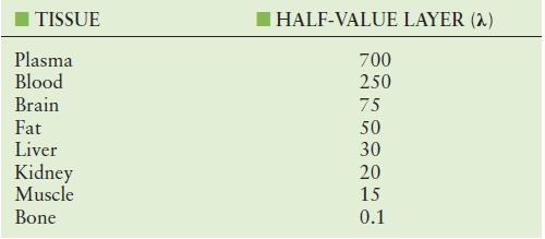
As an ultrasound wave passes farther and farther into tissue, the energy in the ultrasound pulse decreases because of the conversion of that energy into other forms of energy, including heat, and into scattered ultrasound. Conversion can also occur from one ultrasound frequency into another, forming harmonics of the fundamental frequency. Attenuation computations can be easily understood by using the concept of the half-value layer (or half-energy layer). A half-value layer is a layer of tissue thick enough to convert half of the energy in an incoming ultrasound pulse into heat and scattered ultrasound, leaving the remaining half of the ultrasound energy in the pulse as it passes out of the layer. All other attenuation computations can be derived from this concept. Each tissue type has an attenuation rate that can be expressed as a half-value layer (Table 7.4). For most tissues, attenuation increases with ultrasound frequency, so the half-value layer for 2-MHz ultrasound is half as thick as a half-value layer for 1-MHz ultrasound. The wavelength of 2-MHz ultrasound is half as long as the wavelength of 1-MHz ultrasound; therefore, it is most convenient to express the thickness of the half-value layer in wavelengths.
TABLE 7.4 Half-Value Layers for Different Tissues
Attenuation can also be expressed as decibels and nepers. Half-value layers and decibels are defined in units of energy, power, or intensity; nepers are defined in units of amplitude. All are based on the exponential curve, which is the mathematic function that describes the decay of the ultrasound power or energy as ultrasound passes through attenuating tissue. Here, an example using units of half-value layers in wavelengths (HVLW) is presented to simplify understanding.
Imagine that a 15-MHz ultrasound burst with an energy of 64 ergs is sent into a layer of fat that is 0.5 cm thick. The wavelength of the 15-MHz ultrasound in fat is about 0.1 mm [(1.5 mm/μs)/(15 cycles/μs)]. The fat layer is 50 wavelengths thick, that is, 1 HVLW thick. When the burst emerges from the other side, the remaining energy in the burst is 32 ergs. If the burst passes through another 1-HVLW layer, the energy would be 16 ergs. After passing through a third 1-HVLW layer, the burst contains energy of 8 ergs. Every HVLW layer converts half of the energy into heat and scattered ultrasound, leaving half in the remaining beam. After three HVLW layers, only (1/2)3 of the energy remains. Thus, to compute the remaining energy in a burst,
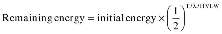
where T is the thickness of the tissue and HVLW is the number of half-value layers through which the ultrasound has passed. A logarithmic plot of the ratio of the remaining to the initial energy versus distance will give a linear (straight line) graph (Fig. 7.14).
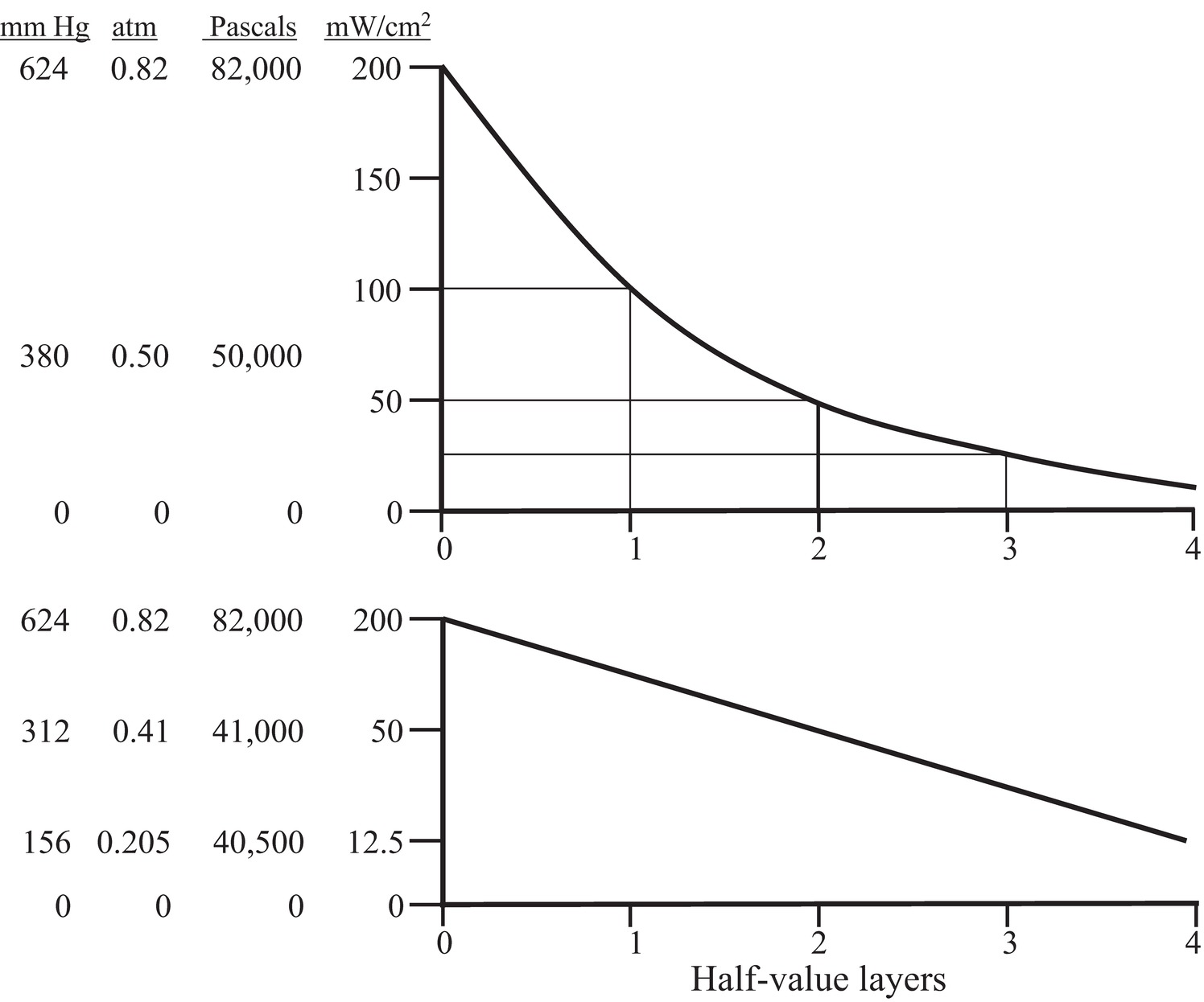
FIGURE 7.14. Half-value layer. As ultrasound is attenuated by any tissue layer, a fraction of the incoming ultrasound is converted to heat. The fraction passing out of the layer is dependent on the thickness and the material. For any material, there is a thickness that will attenuate the ultrasound to a value that is one-half of the incoming energy. The decay in intensity is logarithmic (upper curve). If the log of the energy is displayed on the vertical axis, the decay forms a linear plot (lower curve). In this figure, the vertical axis is plotted as intensity and associated pressure fluctuation amplitude. Intensity is valid only if the beam cross-sectional area remains constant.
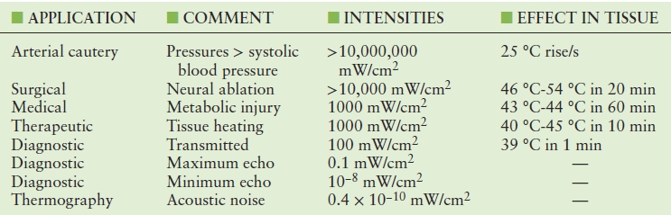
Scattering
The use of ultrasound in medicine spans the range from active tissue ablation to passive acoustic thermography. Between these extremes lies pulse-echo diagnostic ultrasound (Table 7.5). As ultrasound passes through tissue, it crosses boundaries between tissues having different impedances. At each boundary, some ultrasound is reflected, but most passes through the boundary. A voxel is the smallest resolvable volume of tissue and must be analyzed as a single unit; the volume of a voxel is usually about a cubic millimeter. Typically, there are 1,000,000 cells in each voxel of tissue, and within the voxel, the boundaries are the cell walls. Reflections from each of the boundaries travel in a different direction. This is called scattering. Incident ultrasound is scattered in all directions from each voxel. The scattered ultrasound that goes back along the direction of the incident ultrasound beam to the transducer is called backscatter.
TABLE 7.5 Ultrasound Intensities in the Human Body
The backscattered ultrasound from each voxel along the ultrasound beam is the signal that is used to create the ultrasound image and Doppler waveform. That signal must be greater than the natural ultrasound noise emitted from the tissue. Tissues emit ultrasound because they are warm. The intensity of the “thermal noise” from tissue is about 10/1,000,000,000,000,000 W/cm2. This is more easily expressed in scientific notation as 10 × 10−15 W/cm2 or 10 femtowatts/cm2. This can also be expressed in decibels. Decibels always need a reference value; in this case, the maximum SPTA transmit intensity 100 mW/cm2 will be used as a reference. Thermal noise is 10−13 times the reference, or 13 bels or 130 dB below the reference. The backscatter reflectivity of most tissue voxels is less than 0.1% (30 dB) of the incident ultrasound.
Backscatter for different tissue types is compared in the following example. If an ultrasound burst reaches a voxel of interest after passing through 6.5 half-value layers, the ultrasound is attenuated to 1% (0.01) of the original energy in the burst. If the voxel of interest contains liver or muscle cells, about 0.1% of the ultrasound will be reflected back to the transducer as backscatter. If the voxel contains the surface of a bone or a metal surgical clip, 100% (1.0) of the ultrasound will be returned as backscatter. If the voxel contains blood, 0.0001% (60 dB below bone) of the ultrasound will be returned to the transducer as backscatter. As the backscatter passes back along the ultrasound beam pattern to the transducer, it will pass back through 6.5 half-value layers, attenuating the backscattered echo to 1% of the backscattered energy. Reviewing the path of the ultrasound from the voxel of interest: Burst attenuation is 1% (0.01, or 20 dB), reflection from liver produces echo energy of 0.1% (0.001, or 30 dB), and backscatter attenuation is 1% (0.01, or 20 dB) for a total echo strength of (20 + 30 + 20) = 70 dB, compared with the echo that would be produced by a metal plate in contact with the transducer backscattering all of the incident ultrasound. Summarizing for different possible tissues in the voxel of interest, a bone surface echo is 40 dB down, liver is 70 dB down, and blood is 100 dB down.
For an acceptable ultrasound image, the strength of the backscattered echo must be about 100 times (20 dB) greater than the thermal noise. Therefore, if you want the moving speckles of blood in your image to appear brighter than the noise, you need a transmit intensity (100 + 20) = 120 dB greater than thermal noise or (10−14 W/cm2 × 10+12) = 10−2 W/cm2 = 10 mW/cm2. If you use a lower transmit intensity, blood in the voxel of interest will look like noise on the image, and the Doppler spectral waveform will look like noise. If for this example the tissue between the ultrasound transducer is muscle, 6.5 HVLW is about 100 wavelengths (15 cm for 1-MHz ultrasound and 3 cm for 5-MHz ultrasound). If you want to see deeper with 5-MHz ultrasound, you must use a higher transmit intensity (power/area).
Reflection
Some tissue interfaces in the body are large and flat with great impedance changes, such as the diaphragm-pleura interface above the liver. Such interfaces act like mirrors, reflecting entire images into false locations. It is not unusual to see images of liver parenchyma that appear to be located above the diaphragm, where the lung is actually located. It is also easy to view a mirror image of the subclavian artery reflected in the pleura, appearing to be at a depth within the lung. Vascular walls can cause such reflections as well. However, these reflected images are usually displayed at a lower echo intensity than a direct image. Mirror images are more likely to appear in color Doppler imaging than in B-mode imaging because color Doppler is designed to show full brightness even if the signal is weak, whereas B-mode brightness decreases if the echo is weak.
Resolution
One goal in ultrasound B-mode imaging is to achieve the best depth (axial) resolution possible. To ensure that the depth resolution is as small as possible (able to resolve small structures), the shortest possible ultrasound transmit pulse is used (see Fig. 7.9). One factor in resolution is that the burst-echo ultrasound path is folded, so that tissue voxels spaced at 1-mm intervals in depth add 2 mm per voxel to the roundtrip ultrasound path length, and the roundtrip path length is measured by the ultrasound system to determine depth. The ultrasound burst length is the smallest possible resolution division of the roundtrip ultrasound path. Therefore, the voxel dimension along the beam path should be equal to half of the burst length. If the burst length is 2 cycles of ultrasound, then the voxel length should be equal to the wavelength of the ultrasound. Resolution is defined as the closest that two objects can be and still be recognized as separate. Therefore, resolution is the distance between the centers of two bright voxels that have a third, dim voxel between them. The middle low-echo voxel shows that the reflections are separate. Thus, the depth resolution is about equal to the burst length.
This is superior to the lateral resolution, which is about equal to the ultrasound beam pattern width. The beam pattern width is greater than the value of the wavelength times depth divided by aperture. Because depth is almost always greater than aperture, the lateral resolution is poorer than the depth resolution. In a typical case, the focal depth is 80 mm, and the transducer diameter (aperture) is 10 mm. The lateral resolution is greater than eight times the wavelength of the ultrasound. The result is that a small reflecting sphere in the image, which should appear as a bright dot, instead appears as a horizontal dash. If imaged with 5-MHz ultrasound, the dash will appear to be about 0.3 mm deep and 3 mm wide.
Sound Speed Errors
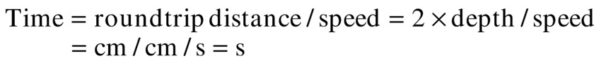
The exact time for an echo to return cannot be determined from the depth of the reflector alone; the time also depends on the speed of travel of the ultrasound in tissue:
Stay updated, free articles. Join our Telegram channel

Full access? Get Clinical Tree


