Fig. 20.1
Electrical and mechanical events of a single cardiac cycle within the left heart (see text for details)
Fig. 20.2
Pressure-volume diagram of a single cardiac cycle (see text for details)
Contractions of the atria begin near the end of ventricular diastole, which is initiated by depolarization of the atrial myocardial cells (sinoatrial node). Atrial depolarization is elicited at the P-wave of the electrocardiogram (Fig. 20.1, ECG lead II). The excitation and subsequent development of tension and shortening of atrial cells cause atrial pressures to rise. Active atrial contraction forces additional volumes of blood into the ventricles (often referred to as atrial kick). The atrial kick can contribute a significant volume of blood toward ventricular preload (approximately 20 %). At normal heart rates, the atrial contractions are considered essential for adequate ventricular filling. As the heart rate increases, atrial filling becomes increasingly important for ventricular filling because the time interval between contractions for passive filling becomes progressively shorter. Atrial fibrillation and/or asynchronized atrioventricular contractions can result in minimal contribution to preload, via the lack of a functional atrial contraction. Throughout diastole, atrial and ventricular pressures are nearly identical due to the open atrioventricular values which offer little or no resistance to blood flow. It should also be noted that contraction and movement of blood out of the atrial appendage (auricle) can be an additional source for increased blood volume.
Ventricular systole begins when the excitation passes from the right atrium, through the atrioventricular node, and through the remainder of the conduction system (His bundle and left and right bundle branches) to cause ventricular myocardial activation. This depolarization of ventricular cells underlies the QRS complex within the ECG (Fig. 20.1). As the ventricular cells contract, intraventricular pressures increase above those in the atria, and the atrioventricular valves abruptly close. Closure of the atrioventricular valves results in the first heart sound, S1 (Fig. 20.1). As pressures in the ventricles continue to rise together in a normally functioning heart, they eventually reach a critical threshold pressure at which the semilunar valves (pulmonary valve and aortic valve) open. The mechanical events of a single cardiac cycle and its pressure-volume relationship are displayed in Fig. 20.2. The normal time period between semilunar valve closures and atrioventricular valve openings is referred to as the isovolumic contraction phase. During this interval, the ventricles can be considered as closed chambers. Ventricular wall tension is greatest just prior to opening of the semilunar valves. Ventricular ejection begins when the semilunar valves open. In early left heart ejection, blood enters the aorta rapidly and causes the pressure within it to rise. Importantly, pressure builds simultaneously in both the left ventricle and the aorta as the ventricular myocardium continues to contract. This period is often referred to as the rapid ejection phase. A similar phenomenon occurs in the right heart; however, the pressures developed and those required to open the pulmonary valve are considerably lower, due to lower resistance within the pulmonary vascular system.
Pressures in the ventricles and outflow vessels (the aorta and pulmonary arteries) ultimately reach maximum peak systolic pressures. Under normal physiologic conditions, the contractile forces in the ventricles diminish after achieving peak systolic pressures. Throughout ejection, there are minimal pressure gradients across the semilunar valves due to their normally large annular diameters. Eventually the ventricular myocardium elicits minimal contraction to a point where intraventricular pressures fall below those in the outflow vessels. This fall in pressures causes the semilunar valves to close rapidly and is associated with the second heart sound, S2 (Fig. 20.1). A quick reversal in both aortic and pulmonary artery pressures is observed at this point, due to back pressure filling the semilunar valve leaflets. The back pressure on the valves causes the incisura or dicrotic notch, which can be detected by local pressure recording (e.g., with a locally placed Millar catheter). After complete closure of these valves, the intraventricular pressure falls rapidly and the ventricular myocardium relaxes. For a brief period, all four cardiac valves are closed, which is commonly referred to as the isovolumetric relaxation phase. Eventually, intraventricular pressure falls below the rising atrial pressures, the atrioventricular valve opens, and a new cardiac cycle is initiated.
20.3 Cardiac Pressure-Volume Curves
Ventricular function can be analyzed and graphically displayed with a pressure-volume diagram. Both systolic and diastolic pressure-volume relationships during a single cardiac cycle are displayed in Fig. 20.2. Pressure-volume assessment of myocardial function on intact myocardium involves multiple factors such as preload, afterload, heart rate, and contractility. The area inside the pressure-volume loop is an estimate of the myocardial energy (work = pressure × volume) utilized for each stroke volume (stroke volume = end-diastolic volume − end-systolic volume). The shape of the normal pressure-volume loop changes with alterations in myocardial compliance, contractility, and valvular or myocardial disease.
Pressure-volume loops are displayed by plotting ventricular pressure (y axis) against ventricular volume (x axis) during a single cardiac cycle (Fig. 20.2). Points and segments along the pressure-volume loop correlate with specific mechanical events of the ventricle. The width of the pressure-volume loop is the stroke volume. Myocardial contractility is represented by the slope of the end-systolic pressure-volume relationship; this relationship defines the maximal pressure generated over time with a given myocardial contractility state. Contractility is proportional to change in pressure over time (dP/dt). The passive ventricular filling during diastole is defined by the end-diastolic pressure-volume relationship, and ventricular compliance is inversely proportional to the slope of the end-diastolic pressure-volume relationship. The effect of heart rate on the pressure-volume relationship cannot be assessed with a single pressure-volume loop. Instead, multiple pressure-volume loops must be obtained to assess effects of heart rate on the pressure-volume loop. By altering variables such as afterload, contractility, and/or preload, the mechanical events and pressure-volume relationship are displayed.
The pressure-volume diagram shows events of a single cardiac cycle (Fig. 20.2):
A:
mitral valve opens; diastole begins.
B:
mitral valve closes; diastole ends.
C:
aortic valve opens; systole begins.
D:
aortic valve closes; systole ends.
A-B:
diastole, ventricular filling.
B-C:
isovolumic contraction.
C-D:
systole, ventricular ejection.
D-A:
isovolumic relaxation.
e:
contractility slope.
20.3.1 Preload
Preload is determined by the end-diastolic ventricular volume; it results from passive and active emptying of the atrium into the ventricle. Factors that affect this relationship, such as mitral stenosis and/or ventricular hypertrophy, will affect preload. The Frank-Starling curve also defines the relationship between preload and stroke volume; as end-diastolic volume increases, the stroke volume increases until the end-diastolic volume gets too excessive to allow proper ventricular contraction (Fig. 20.3). A pressure-volume loop is an alternative way to display the relationship between preload and stroke volume (Fig. 20.4); preload is the volume of blood in the ventricle at the end of diastole (point B in Fig. 20.4). An increase in preload is displayed by a right shift of the end-diastolic volume curve (A-B* in Fig. 20.4). In a normally functioning ventricle, an increase in preload while maintaining normal contractility and afterload results in increased stroke volume (SV* in Fig. 20.4). Excessive preload will not always result in increased stroke volume; excessive overdistention of the ventricle may result in heart failure (Fig. 20.5).
Fig. 20.3
The Frank-Starling relationship. As the end-diastolic volume increases, the cardiac output also increases. Excessive preload may eventually result in decreased cardiac output
Fig. 20.4
Effect of acutely increased preload on the pressure-volume loop. Increasing preload while maintaining normal afterload and contractility results in increased stroke volume (SV*). e contractility line, SV stroke volume
Fig. 20.5
Effect of ventricular failure on the pressure-volume loop. In heart failure, the myocardium compensates its inability to contract by increasing preload in an attempt to maintain stroke volume. Excessive preload eventually leads to worsening of heart failure. e and e* contractility lines, SV stroke volume
20.3.2 Contractility
Contractility is the relative ability of the myocardium to pump blood without changes in preload or afterload; it is influenced by intracellular calcium concentrations, the autonomic nervous system, humoral changes, and/or pharmacologic agents. A sudden increase in contractility with unchanged preload and afterload will result in increased stroke volume by ejecting more volume out of the ventricle (Fig. 20.6). The aortic valve opens at the same pressure and the ventricle ejects blood forward. Increased myocardial contractility forces more blood out of the ventricle during systole, which is displayed by a lower end-systolic volume. Note the change in SV* (Fig. 20.6) with increased contractility; the end-systolic volume is lower due to increased contractility resulting in increased stroke volume. With increased myocardial contractility and unchanged preload, the resulting pressure-volume loop shifts to the left, maintaining normal stroke volume. An increase in contractility is graphically displayed by the increase in the slope of line e* in Fig. 20.6. During ejection, the myocardium contracts from C to D* (Fig. 20.6). During conditions of lower end-diastolic volume, a normal stroke volume may be maintained by increasing contractility. Inotropes such as dopamine and epinephrine will increase contractility, which assists in maintaining adequate stroke volume during low contractility states such as heart failure and/or cardiogenic shock.
Fig. 20.6
Effects of acutely increasing contractility on the pressure-volume loop. Increasing contractility while maintaining normal preload and afterload results in increased stroke volume (SV*). Note the increased slope of the contractility line (e*). The area of loop D* is larger, indicating greater myocardial work per stroke volume. e and e* contractility lines, SV stroke volume
In heart failure, the myocardium has decreased capacity to pump blood and maintain normal cardiac output. Heart failure may be acute (e.g., acute myocardial infarction, acute cardiogenic shock, or fluid overload) or it may be chronic (e.g., chronic congestive heart failure). In progressive heart failure, the myocardium often compensates its inability to contract by increasing preload and decreasing afterload in an attempt to maintain stroke volume (Fig. 20.5).
The increase in preload moves the myocardium up the Frank-Starling curve such that, by increasing end-diastolic volume, normal stroke volume may be maintained. The increase in preload and worsening heart failure eventually leads to ventricular dilatation and venous congestion. During heart failure, sympathetic tone increases as levels of circulating norepinephrine and epinephrine attempt to maintain normal cardiac output by increasing contractility and heart rate. The body’s compensatory mechanism for heart failure may eventually become counterproductive and thus even worsen the situation.
20.3.3 Afterload
Afterload is another vital factor relative to stroke volume and therefore blood pressure. Afterload is most often equated with ventricular wall tension, which is also considered as the pressure the ventricle must overcome to eject a volume of blood past the aortic valve. In most normal clinical situations, afterload is assumed to be proportional to systemic vascular resistance. Wall tension is greatest at the moment just before opening of the aortic valve and can be described by LaPlace’s law:
 where circumferential stress = wall tension, P = intraventricular pressure, r = ventricular radius, and H = wall thickness.
An increase in afterload requires ventricular pressure to increase during isovolumic contraction before the aortic valve opens (Fig. 20.7). Due to the increase in afterload, the ability of the ventricle to eject blood is decreased. This results in decreased stroke volume (SV* in Fig. 20.7a) and increased end-systolic volume (B* in Fig. 20.7b). If afterload remains increased, the myocardium establishes a new steady state that is shifted to the right and stroke volume is restored. A patient with severe aortic stenosis will likely elicit a pressure-volume loop as in Fig. 20.7. The myocardium usually compensates by increasing contractility to maintain adequate stroke volume. Thus, patients with hemodynamically significant aortic stenosis often develop left ventricular hypertrophy.
Fig. 20.7
(a) Effects of acutely increasing afterload on the pressure-volume loop. An increase in afterload, while maintaining normal contractility and preload, results in decreased stroke volume (SV*). A higher pressure is also required before the aortic valve opens (C*). (b) Restoration of stroke volume after increasing afterload. An increase in afterload, while maintaining normal contractility and preload, results in decreased stroke volume (SV*). A higher pressure is also required before the aortic valve opens (C*). e contractility line, SV stroke volume
Afterload may be inversely related to cardiac output. In a dysfunctional myocardium, such as congestive heart failure, stroke volume decreases with increases in afterload. Importantly, increase in afterload also requires the myocardium to expend more energy to eject blood during systole. Conditions such as supravalvular or infravalvular stenoses or obstructions can also impact afterload or wall tension. A clinical example is idiopathic hypertrophic subaortic stenosis (IHSS), a heart condition characterized by significant hypertrophy of the left ventricle and interventricular septum. In turn, the hypertrophied muscle can then obstruct left ventricular outflow of blood during systole, increasing afterload and wall tension.
20.3.4 Sonomicrometry Crystals
A common method for obtaining pressure-volume loops, and the changes observed by varying preload, afterload, or contractility, is to use sonomicrometry crystals for volume measurements in combination with a pressure-sensing catheter placed in the left ventricle. Sonomicrometry consists of piezoelectric crystals that transmit ultrasound signals through tissue to other crystals, where the signal is received; a distance measurement between two given crystals can be determined based upon the travel time of the ultrasound signal and the fiber orientation of the tissue. The piezoelectric (sonomicrometry) crystals function omnidirectionally and act as both receiver and transmitter with as many as 32 peers (in most commonly available systems). Complex, moving 3D geometries can then be modeled using techniques like sonomicrometry array localization. A sonomicrometry crystal can be seen in Fig. 20.8, where it is held in preparation for insertion through the epicardium.
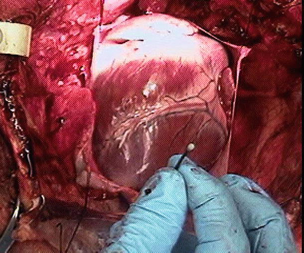
Fig. 20.8
A common sonomicrometry crystal placement. The crystal is shown prior to transmural implantation in a swine heart
Placement of four sonomicrometry crystals transmurally within the left ventricle, as well as the resulting pressure-volume loops, can be viewed online (Online Videos 20.1 and 20.2). The method shown in these supplemental videos places four sonomicrometry crystals—one on the anterior surface, the second on the posterior surface, a third crystal at the base of the left ventricle (superior), and a final crystal at the left ventricular apex (inferior). The placement of the crystals in this pattern creates two distance measurements (anterior-posterior and base-apex) that are measured continuously through the cardiac cycle. By assuming the left ventricle is the shape of an ellipsoid, changes in volume can be continuously estimated.
Traditionally, sonomicrometry has been used to determine cardiac function relative to large research animals (dogs, pigs, sheep, etc.). Both in vivo and in vitro studies can be performed which elucidate global cardiac function under a variety of conditions. Understanding the velocity of ultrasound through tissue is critical to acquiring accurate dimensions in a sonomicrometry system. The velocity of ultrasound is affected by a variety of factors including muscle fiber direction and composition, as well as the contractile state. In most biological tissues, the velocity of sound is approximately 1540 m/s.
A sonomicrometry system can use as few as two transducers but typically employs between six and thirty-two transducers. Transducers are the piezoelectric crystals which are attached to electronics consisting of a pulse generator and a receiver. Distance is measured by energizing the transmitter with a train of high-voltage spikes or square waves (both less than a microsecond in duration) to produce ultrasound. This excites the piezoelectric crystal to begin oscillating at its resonant frequency. This vibratory energy propagates through the medium and eventually comes in contact with piezoelectric crystals acting as receivers. These crystals begin vibrating and generate signals on the order of one millivolt. The piezoelectric signals are amplified and the distances between pairs of crystals are calculated. By monitoring the difference in time from transmission to reception of such signals and knowing the speed of sound through the particular medium, the intercrystal distances can be calculated. With current systems, these computations take less than 1 ms.
In addition to sonomicrometry crystals being used in the manner described, several other types of studies have found sonomicrometry measurements to be helpful. Regional studies have been performed that focus on specific areas of the heart, investigating regional timing and left ventricular shortening [1]. The advent of three-dimensional sonomicrometry, or sonomicrometry array localization, has made possible the detailed study of discrete anatomical points throughout the cardiac cycle [2, 3]. A volume of data now exists describing the motion of valves, papillary muscles, ventricles, and atria. Another application involves tracking mobile components through the heart such as cardiac catheters [4]. We believe that these applications of sonomicrometry are important enough to be described in detail below.
In sonomicrometry array localization, the 3D position of each crystal is calculated from multiple intertransducer distances. This is done using a statistical technique called multidimensional scaling; such assessment gives the experimenter the ability to take the scalar sonomicrometer measurements and generate 3D geometry. Multidimensional scaling generates 3D coordinates for each crystal from a group of chord lengths in the array. By starting with an initial coordinate estimate and applying the Pythagorean theorem, a matrix of estimated distances is generated which corresponds to the actual measured distances. Using an iterative approach, multidimensional scaling then optimizes the value for the distance calculation by minimizing what is called the stress function. If the distances measured between crystals are exact (no measurement error), then one solution with zero stress exists, which represents the intercrystal distances exactly. As measurement error increases, a zero solution to the stress function becomes impossible and the iterations begin seeking a minimum value. The globally minimum stress point defines the optimum 3D configuration. A similar style is used to generate an estimate of the error associated with each distance. The result of this analysis is a 3D moving model with an average error of approximately 2 mm. The advent and description of the feasibility assessment of this technique is described in detail by Ratcliffe et al. [2] and Gorman et al. [3].
The first reported application of this technology described the 3D modeling of the ovine left ventricle and mitral valve. The study involved a 16-transducer array in which three transducers were sutured to the chest wall and the remaining thirteen were placed both epicardially and endocardially on the ventricular wall, the papillary muscles, and the mitral valve. The three crystals attached to the chest wall provided a fixed coordinate system from which whole-body motion could be differentiated from cardiac motion. This study produced 3D depictions of the shape of the mitral annulus throughout the cardiac cycle, as well as quantitative images of ventricular torsion. Such applications open up many possibilities relative to chronic studies focusing on ventricular remodeling following trauma like myocardial infarction.
Another interesting application of sonomicrometry, available due to the development of sonomicrometry array localization, is the cardiac catheter tracking described by Meyer et al. [4]. The system involves placing seven sonomicrometric crystals in the epicardium of an ovine heart and tracking the position of a catheter anywhere from one to five attached crystals. In this system, average distance errors on the order of 1.0 mm were demonstrated by Meyer et al. The clinically relevant endpoint for this tool would be to replace the epicardial transceivers with transceivers mounted in catheters and deployed endocardially in a minimally invasive manner.
20.3.5 Conductance Catheter
Conductance catheters offer an alternative method for obtaining pressure-volume loops. In this method, a catheter is typically equipped with eight electrodes and a pressure lumen. The conductance catheter is placed retrograde across the aortic valve, so that the first electrode is positioned in the left ventricular apex and the eighth electrode is positioned across the aortic valve (Fig. 20.9). The pressure lumen is located within the left ventricle, usually at the distal tip of the conductance catheter.
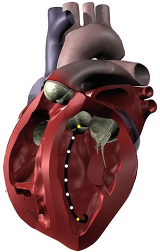
Fig. 20.9
When properly placed within the left ventricle, a conductance catheter spans from the apex to the aortic valve. The outermost electrodes (yellow) produce an electric field, and the inner electrodes (white) measure voltage differences that are related to volume changes within the chamber. A pressure sensor is typically incorporated into the distal tip of the catheter
The outermost electrodes of the conductance catheter produce an electric field, with the remaining electrodes sensing differentials in voltage potential. The use of conductance to measure volume arises from the fact that blood is a good conductor relative to the surrounding myocardium (160 vs. 400 Ω cm) [5]. When the ventricle is in diastole and filled with blood, the conductivity of the chamber will be much higher than during systole. The volume of the heart chamber is then analyzed as a series of conductive cylinders stacked upon each other, with a height predetermined as the distance between the electrodes. A change in the cross-sectional area of one of these cylinders is synonymous with a decrease in blood volume and a change in resistance, which is measured by the sensing electrodes.
The left ventricular volume can then be calculated as a voltage varying with time (V(t)), based upon the distance between the electrodes (L), the specific conductivity of blood (σ), the sum of the conductances that vary with time (G(t)), a dimensionless constant (α), and a correction term (C) [6]:
 The conductance catheter was developed in the early 1980s by Baan et al. [6]. This method has shown reliable left ventricular segmental volumes when compared to cine-CT scans [7] and sonomicrometry crystals. Additionally, the conductance methods could be optimally suited for right ventricular pressure-volume curves [8]. Sonomicrometry methods and angiography require the assumption of an ellipsoid shape for left ventricular measurements; the complex geometric shape of the right ventricle makes these methods ill suited for volume measurements on the right side of the heart.
Both sonomicrometry crystals and conductance catheters are proven techniques for the measurement of left ventricular and aortic root volumes [9]. These technologies are applicable to many different study designs, yet care should be taken to choose the best method based upon the needs of the study. For studies involving complex geometric shapes, a conductance catheter may be the easiest method to obtain absolute volume changes, but a technique such as sonomicrometry array localization may be advantageous if the relative motion of geometric components is of interest.
20.4 Blood Pressure Monitoring
The cardiovascular system is most commonly assessed by monitoring arterial blood pressure. Blood pressure is proportional to the product of cardiac output and systemic vascular resistance:
 where BP = blood pressure, CO = cardiac output, SVR = systemic vascular resistance, HR = heart rate, SV = stroke volume, MAP = mean arterial pressure, SBP = systolic blood pressure, and DBP = diastolic blood pressure. Stroke volume is dependent upon preload, afterload, and contractility (Fig. 20.10).
Fig. 20.10
Blood pressure monitoring which is proportional to the product of cardiac output and systemic vascular resistance. BP blood pressure, CO cardiac output, HR heart rate, SV stroke volume, SVR systemic vascular resistance
Blood pressure can be defined to consist of three components: systolic blood pressure, mean arterial pressure, and diastolic blood pressure. Systolic blood pressure is the peak pressure during ventricular systole, mean arterial pressure is a crucial determinant for adequate perfusion of other major organs, and diastolic blood pressure is the main determinant for myocardial perfusion. Recall that the majority of coronary blood flow occurs during diastole.
Commonly, arterial blood pressure monitoring involves two primary techniques—noninvasive (indirect) and invasive (direct) methods. The decision to utilize either blood pressure monitoring method depends on multiple factors such as: (1) level of a patient’s cardiovascular stability, (2) perceived need for frequent arterial blood samples, (3) relative frequency of blood pressure recordings, and/or (4) type of major surgery or trauma the patient will undergo. One of the advantages of an invasive blood pressure monitor is that it provides continuous, beat-to-beat blood pressures (Online JPG 20.1). Typically, direct arterial blood pressure monitoring is considered to be required when a cardiopulmonary bypass machine is utilized during cardiac surgery. Since there is no pulsatile flow during such surgery, the noninvasive methods to monitor blood pressure cannot be employed. Also, patients with a ventricular assist device may require an invasive arterial monitor, as the noninvasive technique may not provide accurate systemic blood pressures (for more information on ventricular assist devices, see Chap. 39).
20.4.1 Noninvasive Arterial Blood Pressure Monitoring
Noninvasive blood pressure assessment is the most utilized and simplest technique to monitor arterial blood pressure. This technique utilizes a blood pressure cuff and the principle of pulsatile flow. A blood pressure cuff is applied to a limb such as forearm or leg and is inflated to a pressure greater than systolic blood pressure, which stops blood flow distal to the inflated cuff. As the pressure in the cuff is gradually decreased, blood flow through the artery is restored. The change in arterial pressure and blood flow creates oscillations which can be detected by auscultation of Korotkoff sounds and oscillometric methods. For accurate blood pressure measurement, the width of the cuff should be approximately one-third the circumference of the limb. A small, improperly sized cuff will overestimate systolic blood pressure, while a large cuff will underestimate the pressure. The rate of cuff deflation should be slow enough to hear Korotkoff sounds or detect oscillations. Noninvasive blood pressure monitors do not work if there is no pulsatile flow.
The automated method of noninvasive blood pressure monitoring is the oscillometric technique. Most oscillometric blood pressure monitors have oscillotonometers and a microprocessor. The blood pressure cuff is inflated until no oscillation is detected. As the cuff pressure is decreased, flow in the distal blood vessel is restored and amplitude of oscillations increases. A large increase in arterial wave oscillation amplitude is recorded as systolic blood pressure, the peak oscillation as mean arterial pressure, and the sudden decrease in amplitude as diastolic blood pressure (Fig. 20.11). Due to the sensitivity of the monitoring system, the mean arterial pressure is usually the most accurate and reproducible. For more details on such monitoring, refer to Chap. 18.
Fig. 20.11
An example of noninvasive blood pressure monitoring. As blood flow is restored with release of the blood pressure cuff, the arterial wave oscillations increase. The increase in oscillation amplitudes is associated with systolic blood pressure and presence of Korotkoff sounds. The peak of oscillations is associated with mean arterial pressure. Return of oscillations to baseline is diastolic blood pressure and end of Korotkoff sounds
20.4.2 Invasive Arterial Blood Pressure Monitoring
Continuous blood pressure monitoring is best accomplished by direct intra-arterial blood pressure monitoring. Direct pressure monitoring allows for continuous beat-to-beat monitoring of arterial pressure, and the recorded arterial waveform provides temporal information relative to cardiovascular function. Direct pressure monitoring is often employed in clinical settings such as: (1) during major trauma and vascular surgery, (2) in patients with sepsis, (3) during cardiopulmonary bypass where there is no pulsatile flow, (4) in patients with significant cardiovascular instability or fluctuations, and (5) in patients requiring tight blood pressure control, such as hypotension. Further, patients with significant cardiopulmonary disease (i.e., those in an intensive care unit) may require invasive arterial blood pressure monitoring (Table 20.1).
Table 20.1
Accepted indications for direct arterial blood pressure monitor
Major surgery |
Major trauma |
Major vascular (i.e., carotid endarterectomy, aortic aneurysm) |
Cardiopulmonary bypass surgery |
Myocardial dysfunction (i.e., myocardial ischemia/infarct, heart failure, dysrhythmias) |
Uncontrolled/labile blood pressure (i.e., hypertension, hypotension) |
Inaccurate noninvasive monitor (i.e., morbid obesity) |
Sepsis/shock |
Pulmonary dysfunction |
Besides providing blood pressure assessment, the arterial waveform also presents information about cardiovascular function. For example, the upstroke of an arterial waveform correlates with myocardial contractility (dP/dT), while the downstroke gives information relative to peripheral vascular resistance. The position of the dicrotic notch gives insights as to the systemic vascular resistance; a low dicrotic notch position on the arterial waveform may infer low vascular resistance, while a high dicrotic notch usually relates to higher systemic vascular resistance. Furthermore, by integrating the area under the curve of the arterial waveform, the stroke volume may also be estimated.
Direct arterial blood pressure monitoring typically involves cannulation of a peripheral artery and transducing the pressure (Online JPGs 20.2 and 20.3). An indwelling arterial catheter is connected to pressure tubing containing saline, which is then connected to a pressure transducer and monitoring system. Typical transducers contain strain gauges (stretch wires or silicon crystals) that distort with changes in blood pressure. The strain gauges contain a variable resistance transducer and a diaphragm which links the fluid wave to electrical signals. When the transducer diaphragm is distorted, there is a change in voltage across resistors of a Wheatstone bridge circuit (Online JPG 20.4). The transducer is constructed using a circuit so that voltage output can be calibrated proportional to the blood pressure. Standard pressure transducers are calibrated to 5 μV per volt excitation per mmHg [10]. Commonly, the electrical signals from such pressure monitoring systems are filtered, amplified, and displayed on a monitor, thus providing a typical arterial pressure waveform. It is important that the arterial pressure transducer be positioned and calibrated accurately at the level of the heart. Improper transducer height will result in inaccurate blood pressures; if the pressure transducer is positioned too high, the blood pressure is underestimated, while a lower positioned transducer will overestimate the actual blood pressure.
Common sites for intra-arterial cannulation for arterial pressure monitoring are the radial, brachial, axillary, or femoral arteries. Although the ascending aorta is the ideal place to monitor central arterial pressure waveforms, this is not practical in most clinical settings. However, it should be noted that pressure measurements in the more peripheral arteries become distorted when compared to central aortic pressure waveform (Fig. 20.12). Peripherally, the systolic blood pressure may be higher and diastolic blood pressure lower, while the mean arterial pressure is usually similar to central aortic pressure. The pressure waveform becomes more distorted as pressure is measured farther away from the aorta. This distortion is due to a decrease in arterial compliance and reflection and oscillation of the blood pressure waves. For example, an arterial pressure wave monitored from the dorsalis pedis will be significantly different from a central aortic wave when it is graphically displayed (Fig. 20.13). There is also a loss in amplitude or absence of the dicrotic notch, an increase in systolic blood pressure, and a decrease in diastolic blood pressure. One should also be aware of the possible appearance of a reflection wave as the blood pressure is monitored from a peripheral site. Importantly, risks associated with indwelling intra-arterial pressure catheter include thrombosis, emboli, infection, nerve injury, and hematoma.
Fig. 20.12
An example of an arterial blood pressure wave from a typical optimally damped arterial blood pressure waveform. The peak portion of the waveform corresponds to the systolic blood pressure and the trough corresponds with the diastolic blood pressure. The dicrotic notch is associated with closing of the aortic valve. Information about cardiovascular function can be estimated from the waveform. The upstroke correlates with myocardial contractility. The downstroke and position of the dicrotic notch give information about systemic vascular resistance. The stroke volume is estimated by integrating the area under the curve
Fig. 20.13
A typical example of an arterial pressure waveform recorded from the ascending aorta. As the pressure monitoring site is moved more peripherally, the morphology of the waveform changes due to changes in arterial wall compliance as well as oscillation and reflection of the arterial pressure wave. Notice in the dorsalis pedis arterial waveform the absence of the dicrotic notch, overestimation of systolic blood pressure, and underestimation of diastolic pressure. Also note the presence of a small reflection wave
20.4.3 Pressure Transducer System
In clinical settings, arterial and venous blood pressures and waveforms are displayed by utilization of a pressure transducer monitoring system. A typical system includes: (1) an indwelling intravascular catheter, (2) pressure tubing, (3) a pressure transducer, (4) stopcock and flush valve, (5) a high-pressure fluid bag, and (6) a graphical display monitor and microprocessor (Figs. 20.14a, b).
Fig. 20.14
Schematics of a pressure transducer monitoring system (see text for details)
The pressure wave derived from the transducer system is a summation of sine waves at different frequencies and amplitudes. The fundamental frequency (first harmonic) is equal to the heart rate. Therefore, at a heart rate of 120 beats per minute, the fundamental frequency is 2 Hz. Since the first ten harmonics of the fundamental frequency make significant contributions to the arterial waveform [11], frequencies up to 20 Hz make major contributions to the pressure waveform. It is generally considered for most recording systems that the maximum significant frequency in the arterial blood pressure signal is approximately 20 Hz [12].
All materials have a natural frequency, also known as resonant frequency. The natural frequency of the monitoring system is the frequency at which the pressure monitoring system resonates and amplifies the actual blood pressure signal [12, 13]. If the natural frequency of the system is near the fundamental frequency, the blood pressure waveform will be amplified, giving an inaccurate pressure recording. The natural frequency is defined by the following equation [14]:
 where fn = natural frequency, d = tubing diameter, n = viscosity of fluid, L = tubing length, ρ = density of fluid, and V d = transducer fluid volume displacement
In order to increase accuracy of the blood pressure waveform, the natural frequency needs to be increased while the amount of distortion is reduced. The optimal natural frequency should be at least 10 times the fundamental frequency, which is then greater than the tenth harmonic of the fundamental frequency [11, 12]. Therefore, the natural frequency should be greater than 20 Hz. In clinical settings, the input frequency is usually close to the monitoring system’s natural frequency, which ranges from 10–20 Hz. When the input frequency is close to the natural frequency, the system amplifies the actual pressure signal. Ideally, the natural frequency should exceed the maximum significant frequency in a blood pressure signal which is about 20 Hz [12]. An amplified system typically requires damping to minimize distortion; an underdamped system will result in amplification, while an overdamped system will result in reduced amplification.
< div class='tao-gold-member'>
Only gold members can continue reading. Log In or Register to continue
Stay updated, free articles. Join our Telegram channel

Full access? Get Clinical Tree


