2
Fundamentals of EEG Signal Processing
EEG signals are the signatures of neural activities. They are captured by multiple-electrode EEG machines either from inside the brain, over the cortex under the skull, or certain locations over the scalp, and can be recorded in different formats. The signals are normally presented in the time domain, but many new EEG machines are capable of applying simple signal processing tools such as the Fourier transform to perform frequency analysis and equipped with some imaging tools to visualize EEG topographies (maps of the brain activities in the spatial domain).
There have been many algorithms developed so far for processing EEG signals. The operations include, but are not limited to, time-domain analysis, frequency-domain analysis, spatial-domain analysis, and multiway processing. Also, several algorithms have been developed to visualize the brain activity from images reconstructed from only the EEGs. Separation of the desired sources from the multisensor EEGs has been another research area. This can later lead to the detection of brain abnormalities such as epilepsy and the sources related to various physical and mental activities. In Chapter 7 of this book it can be seen that the recent works in brain–computer interfacing (BCI) [1] have been focused upon the development of advanced signal processing tools and algorithms for this purpose.
Modelling of neural activities is probably more difficult than modelling the function of any other organ. However, some simple models for generating EEG signals have been proposed. Some of these models have also been extended to include generation of abnormal EEG signals.
Localization of brain signal sources is another very important field of research [2]. In order to provide a reliable algorithm for localization of the sources within the brain sufficient knowledge about both propagation of electromagnetic waves and how the information from the measured signals can be exploited in separation and localization of the sources within the brain is required. The sources might be considered as magnetic dipoles for which the well-known inverse problem has to be solved, or they can be considered as distributed current sources.
Patient monitoring and sleep monitoring require real-time processing of (up to a few days) long EEG sequences. The EEG provides important and unique information about the sleeping brain. Major brain activities during sleep can be captured using the developed algorithms [3], such as the method of matching pursuits (MPs) discussed [4] later in this chapter.
Epilepsy monitoring, detection, and prediction have also attracted many researchers. Dynamical analysis of a time series together with the application of blind separation of the signal sources has enabled prediction of focal epilepsies from the scalp EEGs. On the other hand, application of time–frequency-domain analysis for detection of the seizure in neonates has paved the way for further research in this area.
In the following sections most of the tools and algorithms for the above objectives are explained and the mathematical foundations discussed. The application of these algorithms to analysis of the normal and abnormal EEGs, however, will follow in later chapters of this book. The reader should also be aware of the required concepts and definitions borrowed from linear algebra, further details of which can be found in Reference [5]. Throughout this chapter and the reminder of this book continuous time is denoted by t and discrete time, with normalized sampling period T = 1, by n.
2.1 EEG Signal Modelling
Most probably the earliest physical model is based on the Hodgkin and Huxley’s Nobel Prize winning model for the squid axon published in 1952 [6–8]. A nerve axon may be stimulated and the activated sodium (Na+) and potassium (K+) channels produced in the vicinity of the cell membrane may lead to the electrical excitation of the nerve axon. The excitation arises from the effect of the membrane potential on the movement of ions, and from interactions of the membrane potential with the opening and closing of voltage-activated membrane channels. The membrane potential increases when the membrane is polarized with a net negative charge lining the inner surface and an equal but opposite net positive charge on the outer surface. This potential may be simply related to the amount of electrical charge Q, using
(2.1) 
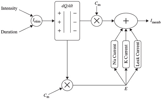
where Q is in terms of coulombs/cm2, Cm is the measure of the capacity of the membrane in units of farads/cm2, and E is in units of volts. In practice, in order to model the action potentials (APs) the amount of charge Q+ on the inner surface (and Q− on the outer surface) of the cell membrane has to be mathematically related to the stimulating current Istim flowing into the cell through the stimulating electrodes. The electrical potential (often called the electrical force) E is then calculated using Equation 2.1. The Hodgkin and Huxley model is illustrated in Figure 2.1. In this figure Imemb is the result of positive charges flowing out of the cell. This current consists of three currents, namely Na, K, and leak currents. The leak current is due to the fact that the inner and outer Na and K ions are not exactly equal.
Hodgkin and Huxley estimated the activation and inactivation functions for the Na and K currents and derived a mathematical model to describe an AP similar to that of a giant squid. The model is a neuron model that uses voltage-gated channels. The space-clamped version of the Hodgkin–Huxley model may be well described using four ordinary differential equations [9]. This model describes the change in the membrane potential (E) with respect to time and is described in Reference [10]. The overall membrane current is the sum of capacity current and ionic current, i.e.
Figure 2.1 The Hodgkin–Huxley excitation model
where Ii is the ionic current and, as indicated in Figure 2.1, can be considered as the sum of three individual components: Na, K, and leak currents:
INa can be related to the maximal conductance  , activation variable aNa, inactivation variable hNa, and a driving force (E − ENa) through
Similarly, IK can be related to the maximal conductance  , activation variable aNa, inactivation variable aK, and a driving force (E − EK) as
and Ileak is related to the maximal conductance  and a driving force (E − E1) as
The changes in the variables aNa, aK, and hNa vary from 0 to 1 according to the following equations:
where α(E) and β(E) are respectively forward and backward rate functions and λt is a temperature-dependent factor. The forward and backward parameters depend on voltage and were empirically estimated by Hodgkin and Huxley as
As stated in the Simulator for Neural Networks and Action Potentials (SNNAP) literature [9], the α(E) and β(E) parameters have been converted from the original Hodgkin–Huxley version to agree with the present physiological practice, where depolarization of the membrane is taken to be positive. In addition, the resting potential has been shifted to –60 mV (from the original 0 mV). These equations are used in the model described in the SNNAP. In Figure 2.2 an AP has been simulated. For this model the parameters are set to Cm = 1.1 uF/cm2,  = 100 ms/cm2,
  = 35 ms/cm2,
  = 0.35 ms/cm2, and ENa = 60 mV.
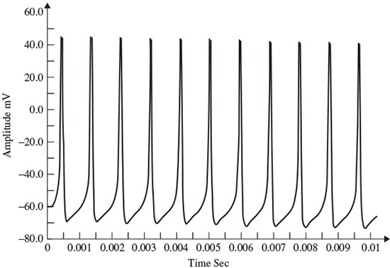
The simulation can run to generate a series of action potentials, as happens in practice in the case of ERP signals. If the maximal ionic conductance of the potassium current,  , is reduced the model will show a higher resting potential. Also, for
  = 16 ms/cm2, the model will begin to exhibit oscillatory behaviour. Figure 2.3 shows the result of a Hodgkin–Huxley oscillatory model with reduced maximal potassium conductance.
The SNNAP can also model bursting neurons and central pattern generators. This stems from the fact that many neurons show cyclic spiky activities followed by a period of inactivity. Several invertebrate as well as mammalian neurons are bursting cells and exhibit alternating periods of high-frequency spiking behaviour followed by a period of no spiking activity.
A simpler model than that due to Hodgkin–Huxley for simulating spiking neurons is the Morris–Lecar model [11]. This model is a minimal biophysical model, which generally exhibits single action potential. This model considers that the oscillation of a slow calcium wave that depolarizes the membrane leads to a bursting state. The Morris–Lecar model was initially developed to describe the behaviour of barnacle muscle cells. The governing equations relating the membrane potential (E) and potassium activation wK to the activation parameters are given as
Figure 2.2 A single AP in response to a transient stimulation based on the Hodgkin–Huxley model. The initiated time is at t = 0.4 ms and the injected current is 80 μA/cm2 for a duration of 0.1 ms. The selected parameters are Cm = 1.2 uF/cm2,  = 100 mS/cm2,
  = 35 ms/cm2,
  = 0.35 ms/cm2, and ENa = 60 mV
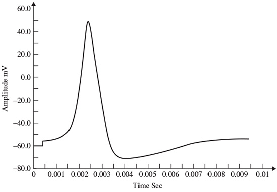
Figure 2.3 The AP from a Hodgkin–Huxley oscillatory model with reduced maximal potassium conductance
where Ii is the combination of three ionic currents, calcium (Ca), potassium (K), and leak (l), and, similar to the Hodgkin–Huxley model, are products of a maximal conductance  , activation components (in such as aCa, wK), and the driving force E. The changes in the potassium activation variable wK), is proportional to a steady-state activation function wK), (E) (a sigmoid curve) and a time-constant function τk(E) (a bell-shaped curve). These functions are respectively defined as
The steady-state activation function aCa(E), involved in calculation of the calcium current, is defined as
Similar to the sodium current in the Hodgkin–Huxley model, the calcium current is an inward current. Since the calcium activation current is a fast process in comparison with the potassium current, it is modelled as an instantaneous function. This means that for each voltage E, the steady-state function aCa(E) is calculated. The calcium current does not incorporate any inactivation process. The activation variable wK here is similar to aK in the Hodgkin–Huxley model, and finally the leak currents for both models are the same [9]. A simulation of the Morris–Lecar model is presented in Figure 2.4.
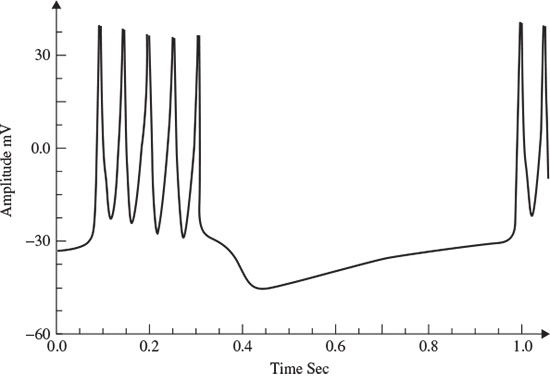
Calcium-dependent potassium channels are activated by intracellular calcium; the higher the calcium concentration the higher the channel activation [9]. For the Morris–Lecar model to exhibit bursting behaviour, the two parameters of maximal time constant and the input current have to be changed [9]. Figure 2.5 shows the bursting behaviour of the Morris–Lecar model. The basic characteristics of a bursting neuron are the duration of the spiky activity, the frequency of the action potentials during a burst, and the duration of the quiescence period. The period of an entire bursting event is the sum of both active and quiescence duration [9].
Neurons communicate with each other across synapses through axon–dendrites or dendrites–dendrites connections, which can be excitatory, inhibitory, or electric [9]. By combining a number of the above models a neuronal network can be constructed. The network exhibits oscillatory behaviour due to the synaptic connection between the neurons.
Figure 2.4 Simulation of an AP within the Morris–Lecar model. The model parameters are: Cm = 22 uF/cm2,  = 3.8 ms/cm2,
  = 8.0 ms/cm2.
  = 1.6 ms/cm2. Eca = 125 mV. Ek = −80 mV, E1 = −60 mV, λt = 0.06, hCa = −1.2, and Sm = 8.8
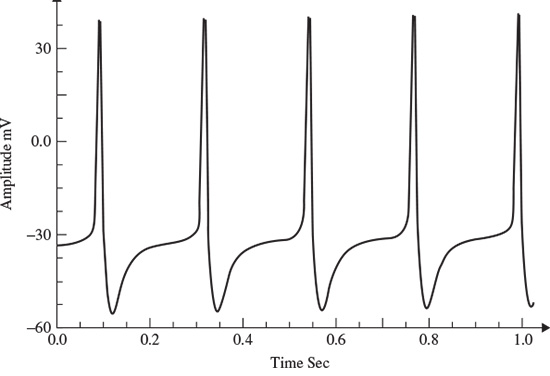
Figure 2.5 An illustration of the bursting behaviour that can be generated by the Morris–Lecar model
A synaptic current is produced as soon as a neuron fires an AP. This current stimulates the connected neuron and may be modelled by an alpha function multiplied by a maximal conductance and a driving force as
Where
and t is the latency or time since the trigger of the synaptic current, u is the time to reach to the peak amplitude, Esyn is the synaptic reversal potential, and  is the maximal synaptic conductance. The parameter u alters the duration of the current while
  changes the strength of the current. This concludes the treatment of the modelling of APs.
As the nature of the EEG sources cannot be determined from the electrode signals directly, many researchers have tried to model these processes on the basis of information extracted using signal processing techniques. The method of linear prediction described in the later sections of this chapter is frequently used to extract a parametric description.
2.1.1 Linear Models
2.1.1.1 Prediction Method
The main objective of using prediction methods is to find a set of model parameters that best describe the signal generation system. Such models generally require a noise-type input. In autoregressive (AR) modelling of signals each sample of a single-channel EEG measurement is defined to be linearly related with respect to a number of its previous samples, i.e.
where ak, k = 1, 2,…, p, are the linear parameters, n denotes the discrete sample time normalized to unity, and x(n) is the noise input. In an autoregressive moving average (ARMA) linear predictive model each sample is obtained based on a number of its previous input and output sample values, i.e.
where bk, k = 1, 2,…, q, are the additional linear parameters. The parameters p and q are the model orders. The Akaike criterion can be used to determine the order of the appropriate model of a measurement signal by minimizing the following equation [12] with respect to the model order:
where i and j represent the assumed AR and MA (moving average) model prediction orders respectively, N is the number of signal samples, and  is the noise power of the ARMA model at the ith and jth stage. Later in this chapter it will be shown how the model parameters are estimated either directly or by employing some iterative optimization techniques.
In a multivariate AR (MVAR) approach a multichannel scheme is considered. Therefore, each signal sample is defined versus both its previous samples and the previous samples of the other channels, i.e. for channel i,
where m represents the number of channels and xi(n) represents the noise input to channel i. Similarly, the model parameters can be calculated iteratively in order to minimize the error between the actual and predicted values [13].
These linear models will be described further later in this chapter and some of their applications are discussed in other chapters. Different algorithms have been developed to find the model coefficients efficiently. In the maximum likelihood estimation (MLE) method [14–16] the likelihood function is maximized over the system parameters formulated from the assumed real, Gaussian distributed, and sufficiently long input signals of approximately 10–20 seconds (consider a sampling frequency of fs = 250 samples/s as often used for EEG recordings). Using Akaike’s method, the gradient of the squared error is minimized using the Newton–Raphson approach applied to the resultant nonlinear equations [16,17]. This is considered as an approximation to the MLE approach. In the Durbin method [18] the Yule–Walker equations, which relate the model coefficients to the autocorrelation of the signals, are iteratively solved. The approach and the results are equivalent to those using a least-squares-based scheme [19]. The MVAR coefficients are often calculated using the Levinson–Wiggins–Robinson (LWR) algorithm [20]. The MVAR model and its application in representation of what is called a direct transfer function (DTF), and its use in the quantification of signal propagation within the brain, will come in the following section. After the parameters are estimated the synthesis filter can be excited with wide-sense stationary noise to generate the EEG signal samples. Figure 2.6 illustrates the simplified system.
2.1.1.2 Prony’s Method
Prony’s method has been previously used to model evoked potentials (EPs) [21,22]. Based on this model an EP, which is obtained by applying a short audio or visual stimulation to the brain, can be considered as the impulse response (IR) of a linear infinite impulse response (IIR) system. The original attempt in this area was to fit an exponentially damped sinusoidal model to the data [23]. This method was later modified to model sinusoidal signals [24]. Prony’s method is used to calculate the linear prediction (LP) parameters. The angles of the poles in the z plane of the constructed LP filter are then referred to the frequencies of the damped sinusoids of the exponential terms used for modelling the data. Consequently, both the amplitude of the exponentials and the initial phase can be obtained following the methods used for an AR model, as follows.
Figure 2.6 A linear model for the generation of EEG signals

Based on the original method the output of an AR system with zero excitation can be considered to be related to its IR as
(2.27) 
where y(n) represents the exponential data samples, p is the prediction order,Wj = Ajejθj, rk = exp[(αk + j2π fk)Ts], Ts is the sampling period normalized to 1, Ak is the amplitude of the exponential, αk is the damping factor, fk is the discrete-time sinusoidal frequency in samples/s, and θj is the initial phase in radians. Therefore, the model coefficients are first calculated using one of the methods previously mentioned in this section, i.e. a = −Y−1ў, where
where a0 = 1. The prediction filter output, i.e. on the basis of Equation 2.27, y(n) is calculated as the weighted sum of p past values of y(n), and the parameters fk and rk are estimated. Hence, the damping factors are obtained as
and the resonance frequencies as
where Re(.) and Im(.) denote the real and imaginary parts of a complex quantity respectively. The wk parameters are calculated using the fact that y(n) = or
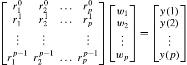
or
In vector form this can be illustrated as Rw = y, where [R]k,l =  , k = 0, 1,…, p – 1, l = 1,…, p, denoting the elements of the matrix in the above equation. Therefore, w = R−1y, assuming R is a full-rank matrix, i.e. there are no repeated poles. Often, this is simply carried out by implementing the Cholesky decomposition algorithm [25]. Finally, using wk, the amplitude and initial phases of the exponential terms are calculated as follows:
and
In the above solution it was considered that the number of data samples N is equal to N = 2p, where p is the prediction order. For cases where N > 2p, a least-squares (LS) solution for w can be obtained as
where (.)H denotes the conjugate transpose. This equation can also be solved using the Cholesky decomposition method. For real data such as EEG signals this equation changes to w = (RTR)−1RTy, where (.)Trepresents the transpose operation. A similar result can be achieved using principal component analysis (PCA) [15].
In the cases where the data are contaminated with white noise the performance of Prony’s method is reasonable. However, for nonwhite noise the noise information is not easily separable from the data and therefore the method may not be sufficiently successful.
In a later chapter of this book it will be seen that, Prony’s algorithm has been used in modelling and analysis of audio and visual evoked potentials (AEP and VEP) [26,27].
2.1.2 Nonlinear Modelling
An approach similar to AR or MVAR modelling in which the output samples are nonlinearly related to the previous samples may be followed based on the methods developed for forecasting financial growth in economical studies. In the generalized autoregressive conditional heteroskedasticity (GARCH) method [28] each sample relates to its previous samples through a nonlinear (or sum of nonlinear) function(s). This model was originally introduced for time-varying volatility (honoured with the Nobel Prize in Economic Sciences in 2003). Nonlinearities in the time series are declared with the aid of the McLeod–Li [29] and BDS (Brock, Dechert, and Scheinkman) tests [30]. However, both tests lack the ability to reveal the actual kind of nonlinear dependency.
Generally, it is not possible to discern whether the nonlinearity is deterministic or stochastic in nature, and nor can a distinction be made between multiplicative and additive dependencies. The type of stochastic nonlinearity can be determined on the basis of the Hseih test [31]. Both additive and multiplicative dependencies can be discriminated by using this test. However, the test itself is not used to obtain the model parameters.
Considering the input to a nonlinear system to be u(n) and the generated signal as the output of such a system to be x(n), a restricted class of nonlinear models suitable for the analysis of such a process is given by
Multiplicative dependence means nonlinearity in the variance, which requires the function h(.) to be nonlinear; additive dependence, on the other hand, means nonlinearity in the mean, which holds if the function g(.) is nonlinear. The conditional statistical mean and variance are respectively defined as
and
where Xn−1 contains all the past information up to time n − 1. The original GARCH(p, q) model, where p and q are the prediction orders, considers a zero mean case, i.e. g(.) = 0. If e(n) represents the residual (error) signal using the above nonlinear prediction system, then
where αj and βj are the nonlinear model coefficients. The second term (first sum) in the right-hand side corresponds to a qth-order moving average (MA) dynamical noise term and the third term (second sum) corresponds to an autoregressive (AR) model of order p. It is seen that the current conditional variance of the residual at time sample n depends on both its previous sample values and previous variances.
Although in many practical applications such as forecasting of stock prices the orders p and q are set to small fixed values such as (p, q) = (1, 1), for a more accurate modelling of natural signals such as EEGs the orders have to be determined mathematically. The prediction coefficients for various GARCH models or even the nonlinear functions g and h are estimated recursively as for the linear ARMA models [28,29].
Clearly, such simple GARCH models are only suitable for multiplicative nonlinear dependence. In addition, additive dependencies can be captured by extending the modelling approach to the class of GARCH-M (GARCH-in-mean) models [32].
Another limitation of the above simple GARCH model is failing to accommodate sign asymmetries. This is because the squared residual is used in the update equations. Moreover, the model cannot cope with rapid transitions such as spikes. Considering these shortcomings, numerous extensions to the GARCH model have been proposed. For example, the model has been extended and refined to include the asymmetric effects of positive and negative jumps such as the exponential GARCH (EGARCH) model [33], the Glosten, Jagannathan, and Runkle GARCH (GJR-GARCH) model [34], the threshold GARCH (TGARCH) model [35], the asymmetric power GARCH (APGARCH) model [36], and the quadratic GARCH (QGARCH) model [37]. In the EGARCH model, for example, the above equation changes to
where log[.] denotes natural logarithm. This logarithmic expression has the advantage of preventing the variance from becoming negative.
In these models different functions for g(.) and h(.) are defined. For example, in the EGARCH model proposed by Glosten et al. [34] h(n) is iteratively computed as
where b, α1, α2, and k are constants and η(n) is an indicator function that is zero when u(n) is negative and one otherwise.
Despite modelling the signals, the GARCH approach has many other applications. In some recent works [38] the concept of GARCH modelling of covariance is combined with Kalman filtering to provide a more flexible model with respect to space and time for solving the inverse problem. There are several alternatives for solution to the inverse problem. Many approaches fall into the category of constrained least-squares methods employing Tikhonov regularization [39]. Localization of the sources within the brain using the EEG information is as an example. This approach has become known as low-resolution electromagnetic tomography (LORETA) [40]. Among numerous possible choices for the GARCH dynamics, the EGARCH [33] has been used to estimate the variance parameter of the Kalman filter sequentially.
The above methods are used to model the existing data, but to generate the EEG signals accurately a very complex model that exploits the physiological dynamics and various mental activities of the brain has to be constructed. Such a model should also incorporate the changes in the brain signals due to abnormalities and the onset of diseases. The next section considers the interaction among various brain components to establish a more realistic model for generation of the EEG signals.
2.1.3 Generating EEG Signals Based on Modelling the Neuronal Activities
The objective in this section is to introduce some established models for generating normal and some abnormal EEGs. These models are generally nonlinear, some have been proposed [41] for modelling a normal EEG signal and some others for the abnormal EEGs.
A simple distributed model consisting of a set of simulated neurons, thalamocortical relay cells, and interneurons was proposed [42,43] that incorporates the limited physiological and histological data available at that time. The basic assumptions were sufficient to explain the generation of the alpha rhythm, i.e. the EEGs within the frequency range of 8–13 Hz.
A general nonlinear lumped model may take the form shown in Figure 2.7. Although the model is analogue in nature, all the blocks are implemented in a discrete form. This model can take into account the major characteristics of a distributed model and it is easy to investigate the result of changing the range of excitatory and inhibitory influences of thalamocortical relay cells and interneurons.
Figure 2.7 A nonlinear lumped model for generating the rhythmic activity of the EEG signals; he(t) and hi(t) are the excitatory and inhibitory postsynaptic potentials, f(v) is normally a simplified nonlinear function, and the Cis are respectively the interaction parameters representing the interneurons and thalamocortical neurons
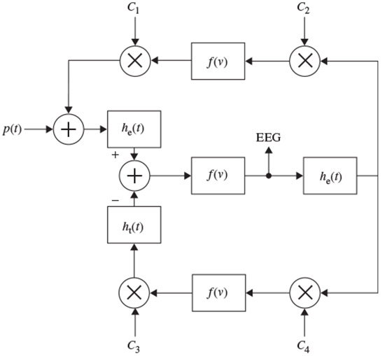
In this model [42] there is a feedback loop including the inhibitory postsynaptic potentials, the nonlinear function, and the interaction parameters C3 and C4. The other feedback includes mainly the excitatory potentials, nonlinear function, and the interaction parameters C1 and C2. The role of the excitatory neurons is to excite one or two inhibitory neurons. The latter, in turn, serve to inhibit a collection of excitatory neurons. Thus, the neural circuit forms a feedback system. The input p(t) is considered as a white noise signal. This is a general model; more assumptions are often needed to enable generation of the EEGs for the abnormal cases. Therefore, the function f(v) may change to generate the EEG signals for different brain abnormalities. Accordingly, the Ci coefficients can be varied. In addition, the output is subject to environment and measurement noise. In some models, such as the local EEG model (LEM) [42] the noise has been considered as an additive component in the output.
Figure 2.8 shows the LEM model. This model uses the formulation by Wilson and Cowan [44] who provided a set of equations to describe the overall activity (not specifically the EGG) in a cartel of excitatory and inhibitory neurons having a large number of interconnections [45]. Similarly, in the LEM the EEG rhythms are assumed to be generated by distinct neuronal populations, which possess frequency selective properties. These populations are formed by the interconnection of the individual neurons and are assumed to be driven by a random input. The model characteristics, such as the neural interconnectivity, synapse pulse response, and threshold of excitation, are presented by the LEM parameters. The changes in these parameters produce the relevant EEG rhythms.
Figure 2.8 The local EEG model (LEM). The thalamocortical relay neurons are represented by two linear systems having impulse responses he(t), on the upper branch, and the inhibitory postsynaptic potential represented by hi(t). The nonlinearity of this system is denoted by fe(v), representing the spike-generating process. The interneuron activity is represented by another linear filter he(t) in the lower branch, which generally can be different from the first linear system, and a nonlinearity function fi(v). Ce and Ci represent respectively the number of interneuron cells and the thalamocortical neurons
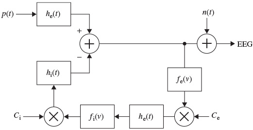
In Figure 2.8, as in Figure 2.7, the notation ‘e’ and ‘i’ refer to excitatory and inhibitory respectively. The input p(t) is assumed to result from the summation of a randomly distributed series of random potentials which drive the excitatory cells of the circuit, producing the ongoing background EEG signal. Such signals originate from other deeper brain sources within the thalamus and brain stem and constitute part of the ongoing or spontaneous firing of the central nervous system (CNS). In the model, the average number of inputs to an inhibitory neuron from the excitatory neurons is designated by Ce and the corresponding average number from inhibitory neurons to each individual excitatory neuron is Ci. The difference between two decaying exponentials is used for modelling each postsynaptic potential he or hi:
where A, B, ak, and bk are constant parameters, which control the shape of the pulse waveforms. The membrane potentials are related to the axonal pulse densities via the static threshold functions fe and fi. These functions are generally nonlinear, but to ease the manipulations they are considered linear for each short time interval. Using this model, the normal brain rhythms, such as the alpha wave, are considered as filtered noise.
The main problem with such a model is due to the fact that only a single-channel EEG is generated and there is no modelling of interchannel relationships. Therefore, a more accurate model has to be defined to enable simulation of a multichannel EEG generation system. This is still an open question and remains an area of research.
2.2 Nonlinearity of the Medium
The head as a mixing medium combines EEG signals which are locally generated within the brain at the sensor positions. As a system, the head may be more or less susceptible to such sources in different situations. Generally, an EEG signal can be considered as the output of a nonlinear system, which may be characterized deterministically.
The changes in brain metabolism as a result of biological and physiological phenomena in the human body can change the mixing process. Some of these changes are influenced by the activity of the brain itself. These effects make the system nonlinear. Analysis of such a system is very complicated and up to now nobody has fully modelled the system to aid in the analysis of brain signals.
On the other hand, some measures borrowed from chaos theory and analysis of the dynamics of time series such as dissimilarity, attractor dimension, and largest Lyapunov exponents (LLE) can characterize the nonlinear behaviour of EEG signals. These concepts are discussed in Section 2.7 and some of their applications are given in Chapter 5.
2.3 Nonstationaritys
Nonstationarity of the signals can be quantified by measuring some statistics of the signals at different time lags. The signals can be deemed stationary if there is no considerable variation in these statistics.
Although generally the multichannel EEG distribution is considered as multivariate Gaussian, the mean and covariance properties generally change from segment to segment. Therefore EEGs are considered stationary only within short intervals, i.e. quasistationarity. This Gaussian assumption holds during a normal brain condition, but during mental and physical activities this assumption is not valid. Some examples of nonstationarity of the EEG signals can be observed during the change in alertness and wakefulness (where there are stronger alpha oscillations), during eye blinking, during the transitions between various ictal states, and in the event-related potential (ERP) and evoked potential (EP) signals.
The change in the distribution of the signal segments can be measured in terms of both the parameters of a Gaussian process and the deviation of the distribution from Gaussian. The non-Gaussianity of the signals can be checked by measuring or estimating some higher-order moments such as skewness, kurtosis, negentropy, and Kulback–Laibler (KL) distance.
Skewness is a measure of symmetry or, more precisely, the lack of symmetry of the distribution. A distribution, or data set, is symmetric if it looks the same to the left and right of the centre point. The skewness is defined for a real signal as
(2.43) 
where μ and θ are the mean and standard deviation respectively, and E denotes statistical expectation. If the distribution is more to the right of the mean point the skewness is negative, and vice versa. For a symmetric distribution such as Gaussian, the skewness is zero.
Kurtosis is a measure of whether the data are peaked or flat relative to a normal distribution; i.e. data sets with high kurtosis tend to have a distinct peak near the mean, decline rather rapidly, and have heavy tails. Data sets with low kurtosis tend to have a flat top near the mean rather than a sharp peak. A uniform distribution would be the extreme case. The kurtosis for a real signal x(n) is defined as
where mi [x(n)] is the ith central moment of the signal x(n), i.e. mi [x(n)] = E[(x(n) − μ)i]. The kurtosis for signals with normal distributions is three. Therefore, an excess or normalized kurtosis is often used and defined as
(2.45) 
which is zero for Gaussian distributed signals. Often the signals are considered ergodic; hence the statistical averages can be assumed identical to time averages and so can be estimated with time averages.
The negentropy of a signal x(n) [46] is defined as
where, xGauss(n) is a Gaussian random signal with the same covariance as x(n) and H(.) is the differential entropy [47], defined as
and p[x(n)] is the signal distribution. Negentropy is always nonnegative.
The KL distance between two distributions p1 and p2 is defined as
It is clear that the KL distance is generally asymmetric, therefore by changing the position of p1 and p2 in this equation the KL distance changes. The minimum of the KL distance occurs when p1(x1(n)) = p2(x2(n)).
2.4 Signal Segmentation
Often it is necessary to label the EEG signals by segments of similar characteristics that are particularly meaningful to clinicians and for assessment by neurophysiologists. Within each segment, the signals are considered statistically stationary, usually with similar time and frequency statistics. As an example, an EEG recorded from an epileptic patient may be divided into three segments of preictal, ictal, and postictal segments. Each may have a different duration. Figure 2.9 represents an EEG sequence including all the above segments.
Figure 2.9 An EEG set of tonic–clonic seizure signals including three segments of preictal, ictal, and postictal behaviour
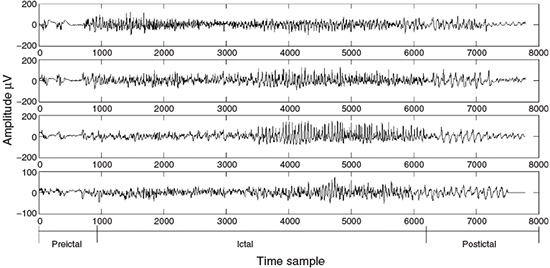
In segmentation of an EEG the time or frequency properties of the signals may be exploited. This eventually leads to a dissimilarity measurement denoted as d(m) between the adjacent EEG frames, where m is an integer value indexing the frame and the difference is calculated between the m and (m – 1)th (consecutive) signal frames. The boundary of the two different segments is then defined as the boundary between the m and (m – 1)th frames provided d(m) > ηT, and ηT is an empirical threshold level. An efficient segmentation is possible by highlighting and effectively exploiting the diagnostic information within the signals with the help of expert clinicians. However, access to such experts is not always possible and therefore algorithmic methods are required.
A number of different dissimilarity measures may be defined based on the fundamentals of digital signal processing. One criterion is based on the autocorrelations for segment m, defined as
The autocorrelation function of the mth length N frame for an assumed time interval n, n + 1, . . . , n + (N – 1) can be approximated as
Then the criterion is set to
A second criterion can be based on higher-order statistics. The signals with more uniform distributions such as normal brain rhythms have a low kurtosis, whereas seizure signals or event related potentials (ERP signals) often have high kurtosis values. Kurtosis is defined as the fourth-order cumulant at zero time lags and is related to the second- and fourth- order moments as given in Equations (2.43) to (2.45). A second level discriminant d2(m) is then defined as
where m refers to the mth frame of the EEG signal x(n). A third criterion is defined from the spectral error measure of the periodogram. A periodogram of the mth frame is obtained by discrete time Fourier transforming of the correlation function of the EEG signal
where  (., m) is the autocorrelation function for the mth frame as defined above. The criterion is then defined based on the normalized periodogram as
The test window sample autocorrelation for the measurement of both d1 (m) and d3 (m)) can be updated through the following recursive equation over the test windows of size N:
and thereby computational complexity can be reduced in practice. A fourth criterion corresponds to the error energy in autoregressive (AR)-based modelling of the signals. The prediction error in the AR model of the mth frame is simply defined as
(2.56) 
where p is the prediction order and ak(m), k = 1, 2,…, p, are the prediction coefficients. For certain p the coefficients can be found directly (e.g. Durbin’s method) in such a way as to minimize the error (residual) signal energy. In this approach it is assumed that the frames of length N are overlapped by one sample. The prediction coefficients estimated for the (m – 1)th frame are then used to predict the first sample in the mth frame, which is denoted as ê(1, m). If this error is small, it is likely that the statistics of the mth frame are similar to those of the (m – 1)th frame. On the other hand, a large value is likely to indicate a change. An indicator for the fourth criterion can then be the differencing of this prediction signal, which gives a peak at the segment boundary, i.e.
(2.57) 
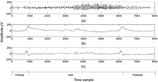
where ∇m(.) denotes the gradient with respect to m, approximated by a first-order difference operation. Figure 2.10 shows the residual and the gradient defined in Equation 2.57
Finally, a fifth criterion d5(m) may be defined by using the AR-based spectrum of the signals in the same way as the short-term frequency transform (STFT) for d3(m). The above AR model is a univariate model, i.e. it models a single-channel EEG. A similar criterion may be defined when multichannel EEGs are considered [20]. In such cases a multivariate AR (MVAR) model is analysed. The MVAR can also be used for characterization and quantification of the signal propagation within the brain and is discussed in the next section.
Although the above criteria can be effectively used for segmentation of EEG signals, better systems may be defined for the detection of certain abnormalities. In order to do that, the features that best describe the behaviour of the signals have to be identified and used. Therefore the segmentation problem becomes a classification problem for which different classifiers can be used.
Figure 2.10 (a) An EEG seizure signal including preictal ictal and postictal segments, (b) the error signal, and (c) the approximate gradient of the signal, which exhibits a peak at the boundary between the segments. The number of prediction coefficients p = 12
2.5 Signal Transforms and Joint Time–Frequency Analysis
If the signals are statistically stationary it is straightforward to characterize them in either the time or frequency domains. The frequency-domain representation of a finite-length signal can be found by using linear transforms such as the (discrete) Fourier transform (DFT), (discrete) cosine transform (DCT), or other semi-optimal transform, which have kernels independent of the signal. However, the results of these transforms can be degraded by spectral smearing due to the short-term time-domain windowing of the signals and fixed transform kernels. An optimal transform such as the Karhunen–Loéve transform (KLT) requires complete statistical information, which may not be available in practice.
Parametric spectrum estimation methods such as those based on AR or ARMA modelling can outperform the DFT in accurately representing the frequency-domain characteristics of a signal, but they may suffer from poor estimation of the model parameters mainly due to the limited length of the measured signals. For example, in order to model the EEGs using an AR model, accurate values for the prediction order and coefficients are necessary. A high prediction order may result in splitting the true peaks in the frequency spectrum and a low prediction order results in combining peaks in close proximity in the frequency domain.
For an AR model of the signal x(n) the error or driving signal is considered to be zero mean white noise. Therefore, by applying a z-transform to Equation 2.56, dropping the block index m, and replacing z by ejω gives
where, E(ω) = Kω (constant) is the power spectrum of the white noise and Xp(ω) is used to denote the signal power spectrum. Hence,
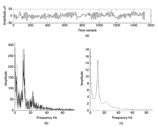
and the parameters Kω, ak, k = 1,…, p, are the exact values. In practical AR modelling these would be estimated from the finite length measurement, thereby degrading the estimate of the spectrum. Figure 2.11 provides a comparison of the spectrum of an EEG segment of approximately 1550 samples of a single-channel EEG using both DFT analysis and AR modelling.
The fluctuations in the DFT result as shown in Figure 2.11(b) are a consequence of the statistical inconsistency of periodogram-like power spectral estimation techniques. The result from the AR technique (Figure 2.11(c)) overcomes this problem provided the model fits the actual data. EEG signals are often statistically nonstationary, particularly where there is an abnormal event captured within the signals. In these cases the frequency-domain components are integrated over the observation interval and do not show the characteristics of the signals accurately. A time–frequency (TF) approach is the solution to the problem.
In the case of multichannel EEGs, where the geometrical positions of the electrodes reflect the spatial dimension, a space–time–frequency (STF) analysis through multiway processing methods has also become popular [48]. The main concepts in this area, together with the parallel factor analysis (PARAFAC) algorithm, will be reviewed in Chapter 7 where its major applications will be discussed.
Figure 2.11 Single-channel EEG spectrum: (a) a segment of the EEG signal with a dominant alpha rhythm, (b) the spectrum of the signal in (a) using the DFT, and (c) the spectrum of the signal in (a) using a 12-order AR model
The short-time Fourier transform (STFT) is defined as the discrete-time Fourier transform evaluated over a sliding window. The STFT can be performed as
where the discrete-time index n refers to the position of the window w(n). Analogous with the periodogram, a spectrogram is defined as
Based on the uncertainity principle, i.e.  where
where  of and
  of are respectively the time- and frequency-domain variances, perfect resolution cannot be achieved in both time and frequency domains. Windows are typically chosen to eliminate discontinuities at block edges and to retain positivity in the power spectrum estimate. The choice also impacts upon the spectral resolution of the resulting technique, which, put simply, corresponds to the minimum frequency separation required to resolve two equal amplitude frequency components [49].
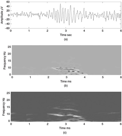
Figure 2.12 shows the TF representation of an EEG segment during the evolution from preictal to ictal and to postictal stages. In this figure the effect of time resolution has been illustrated using a Hanning window of different durations of 1 and 2 seconds. Importantly, in this figure the drift in frequency during the ictal period is observed clearly.
Figure 2.12 TF representation of an epileptic waveform (a) for different time resolutions using a Hanning window of (b) 1 ms and (c) 2 ms duration
2.5.1 Wavelet Transform
The wavelet transform (WT) is another alternative for a time–frequency analysis. There is already a well-established literature detailing the WT, such as References [50] and [51]. Unlike the STFT, the time–frequency kernel for the WT-based method can better localize the signal components in time–frequency space. This efficiently exploits the dependency between time and frequency components. Therefore, the main objective of introducing the WT by Morlet [50] was likely to have a coherence time proportional to the sampling period. To proceed, consider the context of a continuous time signal.
2.5.1.1 Continuous Wavelet Transform
The Morlet–Grossmann definition of the continuous wavelet transform for a one-dimensional signal f(t) is
where (.)* denotes the complex conjugate, ψ(t) is the analysing wavelet, a(> 0) is the scale parameter (inversely proportional to frequency), and b is the position parameter. The transform is linear and is invariant under translations and dilations, i.e.
and
The last property makes the wavelet transform very suitable for analysing hierarchical structures. It is similar to a mathematical microscope with properties that do not depend on the magnification. Consider a function W(a,b) which is the wavelet transform of a given function f(t). It has been shown [52,53] that f(t) can be recovered according to
where
Although often it is considered that ψ(t) = φ(t), other alternatives for φ(t) may enhance certain features for some specific applications [54]. The reconstruction of f(t) is subject to having Cφ defined (admissibility condition). The case ψ(t) = φ(t) implies  i.e. the mean of the wavelet function is zero.
2.5.1.2 Examples of Continuous Wavelets
Different waveforms/wavelets/kernels have been defined for the continuous wavelet transforms. The most popular ones are given below.
Morlet’s wavelet is a complex waveform defined as
This wavelet may be decomposed into its constituent real and imaginary parts as
where b0 is a constant, and it is considered that b0 > 0 to satisfy the admissibility condition. Figure 2.13 shows respectively the real and imaginary parts.
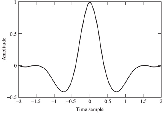
The Mexican hat defined by Murenzi et al. [51] is
which is the second derivative of a Gaussian waveform (see Figure 2.14).
2.5.1.3 Discrete-Time Wavelet Transform
In order to process digital signals a discrete approximation of the wavelet coefficients is required. The discrete wavelet transform (DWT) can be derived in accordance with the sampling theorem if a frequency band-limited signal is processed.
The continuous form of the WT may be discretized with some simple considerations on the modification of the wavelet pattern by dilation. Since generally the wavelet function ψ(t) is not band-limited, it is necessary to suppress the values of the frequency components above half the sampling frequency to avoid aliasing (overlapping in frequency) effects.
Figure 2.13 Morlet’s wavelet: (a) real and (b) imaginary parts
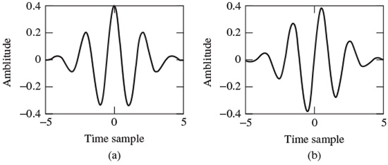
Figure 2.14 Mexican hat wavelet
A Fourier space may be used to compute the transform scale-by-scale. The number of elements for a scale can be reduced if the frequency bandwidth is also reduced. This requires a band-limited wavelet. The decomposition proposed by Littlewood and Paley [55] provides a very informative illustration of the reduction of elements scale-by-scale. This decomposition is based on an stagewise dichotomy of the frequency band. The associated wavelet is well localized in Fourier space, where it allows a reasonable analysis to be made, although not in the original space. The search for a discrete transform that is well localized in both spaces leads to a multiresolution analysis.
2.5.1.4 Multiresolution Analysis
Multiresolution analysis results from the embedded subsets generated by the interpolations (or down-sampling and filtering) of the signal at different scales. A function f(t) is projected at each step j on to the subset Vj. This projection is defined by the scalar product cj(k) of f(t) with the scaling function φ(t), which is dilated and translated as
where ‹.,.›denotes an inner product and ϕ(t) has the property
where the right-hand side is convolution of h and ϕ. By taking the Fourier transform of both sides,
where H(ω) and Φ(ω) are the Fourier transforms of h(t) and ϕ(t) respectively. For a discrete frequency space (i.e. using the DFT) the above equation permits the computation of the wavelet coefficient Cj+1(k) from Cj(k) directly. If a start is made from C0(k) and all Cj(k), with j > 0, are computed without directly computing any other scalar product, then
where k is the discrete frequency index and N is the signal length.
At each step, the number of scalar products is divided by two and consequently the signal is smoothed. Using this procedure the first part of a filter bank is built up. In order to restore the original data, Mallat uses the properties of orthogonal wavelets, but the theory has been generalized to a large class of filters by introducing two other filters  and
and  also called conjugate filters. The restoration is performed with
where wj+1 (.) are the wavelet coefficients at the scale j + 1 defined later in this section. For an exact restoration, two conditions have to be satisfied for the conjugate filters:
Anti-aliasing condition:
Exact restoration:
(2.77) 
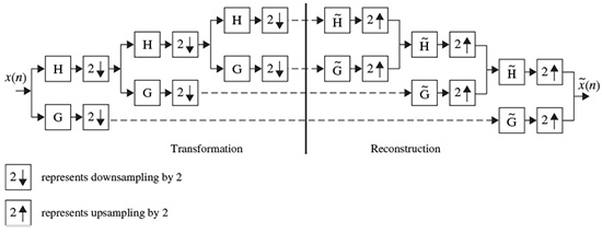
In the decomposition, the input is successively convolved with the time domain forms of the two filters H (low frequencies) and G (high frequencies). Each resulting function is decimated by suppression of one sample out of two. The high-frequency signal is left untouched, and the decomposition continues with the low-frequency signal (left-hand side of Figure 2.15). In the reconstruction, the sampling is restored by inserting a zero between each sample; then the conjugate filters  and
and  are applied, the resulting outputs are added and the result is multiplied by 2. Reconstruction continues to the smallest scale (right-hand side of Figure 2.15). Orthogonal wavelets correspond to the restricted case where
and
Figure 2.15 The filter bank associated with the multiresolution analysis
It can easily be seen that this set satisfies the two basic relations (2.72) and (2.73). Among various wavelets, Daubechie’s wavelets are the only compact solutions to satisfy the above conditions. For biorthogonal wavelets, then
and
The relations (2.76) and (2.77) have also to be satisfied. A large class of compact wavelet functions can be used. Many sets of filters have been proposed, especially for coding [56]. It has been shown that the choice of these filters must be guided by the regularity of the scaling and the wavelet functions. The complexity is proportional to N. The algorithm provides a pyramid of N elements.
2.5.1.5 The Wavelet Transform using the Fourier Transform
Consider the scalar products c0(k) = 〈f(t) ϕ (t – k)〉 for continuous wavelets. If ϕ(t) is band-limited to half of the sampling frequency, the data can be correctly sampled. The data at the resolution j = 1 are
and the set c1 (k) can be computed from c0(k) with a discrete-time filter with the frequency response H(ω)
and for  ω and
ω and  integer m
Therefore, the coefficients at the next scale can be found from
The cut-off frequency is reduced by a factor 2 at each step, allowing a reduction of the number of samples by this factor. The wavelet coefficients at the scale j + 1 are
and can be computed directly from Cj by
where G is the following discrete-time filter:
and for ∀ω and ∀ integer m
The frequency band is also reduced by a factor of two at each step. These relationships are also valid for DWT, following Section 2.5.1.4.
2.5.1.6 Reconstruction
The reconstruction of the data from its wavelet coefficients can be performed step-by-step, starting from the lowest resolution. At each scale,
when a search is made for Cj knowing Cj+1, Wj+1, h, and g. Then Cj(ω) is restored by minimizing
using a least squares estimator. Ph(ω) and Pg(ω) are weight functions that permit a general solution to the restoration of Cj(ω) . The relationship of Cj(ω) is in the form of
where the conjugate filters have the expressions
(2.97) 
(2.98) 
It is straightforward to see that these filters satisfy the exact reconstruction condition given in Equation 2.77. In fact, Equations (2.97) and (2.98) give the general solutions to this equation. In this analysis, the Shannon sampling condition is always respected. No aliasing exists, so that the antialiasing condition (2.76) is not necessary. The denominator is simplified if
This corresponds to the case where the wavelet is the difference between the squares of two resolutions:
The reconstruction algorithm then carries out the following steps:

 and.
and. + Cj
+ Cj and gives the coefficients Cj−1.
The use of a band-limited scaling function allows a reduction of sampling at each scale and limits the computation complexity.
The wavelet transform has been widely used in EEG signal analysis. Its application to seizure detection, especially for neonates, modelling of the neuron potentials, and the detection of evoked potentials (EP) and event-related potentials (ERP) will be discussed in the corresponding chapters of this book.
2.5.2 Ambiguity Function and the Wigner–Ville Distribution
The ambiguity function for a continuous time signal is defined as
This function has its maximum value at the origin as
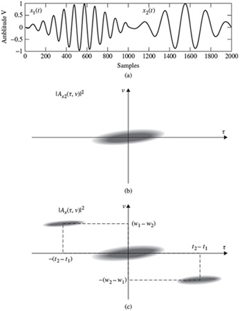
As an example, if a continuous time signal is considered to consist of two modulated signals with different carrier frequencies such as
The ambiguity function Ax(τ,v) will be in the form of
This concept is very important in the separation of signals using the TF domain. This will be addressed in the context of blind source separation (BSS) later in this chapter.
Figure 2.16 demonstrates this concept.
The Wigner–Ville frequency distribution of a signal x(t) is then defined as the twodimensional Fourier transform of the ambiguity function
which changes to the dual form of the ambiguity function as
A quadratic form for the TF representation with the Wigner–Ville distribution can also be obtained using the signal in the frequency domain as
The Wigner–Ville distribution is real and has very good resolution in both the time and frequency domains. Also it has time and frequency support properties; i.e. if x(t) = 0 for |t| > t0, then XWV(t, ω) = 0 for |t| > t0, and if X(ω) = 0 for |ω| > ω0, then XWV(t, ω) = for |ω| > ω0. It has also both time-marginal and frequency-marginal conditions of the form
Figure 2.16 (a) A segment of a signal consisting of two modulated components, (b) an ambiguity function for x1(t) only, and (c) the ambiguity function for x(t) = x1(t) + x2(t)
and
If x(t) is the sum of two signals x1(t) and x2(t), i.e. x(t) = x1(t) + x2(t), the Wigner–Ville distribution of x(t) with respect to the distributions of x1(t) and x2(t) will be
where Re[.] denotes the real part of a complex value and
It is seen that the distribution is related to the spectra of both auto- and cross-correlations. A pseudo Wigner–Ville distribution (PWVD) is defined by applying a window function, w(τ), centred at τ = 0 to the time-based correlations, i.e.
In order to suppress the undesired cross-terms the two-dimensional WV distribution may be convolved with a TF-domain window. The window is a two-dimensional lowpass filter, which satisfies the time and frequency marginal (uncertainty) conditions, as described earlier. This can be performed as
where
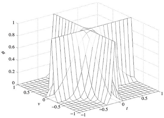
and ϕ(., .) is often selected from a set of well-known signals, the so-called Cohen’s class. The most popular member of Cohen’s class of functions is the bell-shaped function defined as
A graphical illustration of such a function can be seen in Figure 2.17. In this case the distribution is referred to as a Choi–Williams distribution.
The application of a discrete time form of the Wigner–Ville distribution to BSS will be discussed later in this chapter and its application to seizure detection will be briefly explained in Chapter 4. To improve the distribution a signal-dependent kernel may also be used [57].
2.6 Coherency, Multivariate Autoregressive (MVAR) Modelling, and Directed Transfer Function (DTF)
In some applications such as in detection and classification of finger movement, it is very useful to establish how the associated movement signals propagate within the neural network of the brain. As will be shown in Chapter 7, there is a consistent movement of the source signals from the occipital to temporal regions. It is also clear that during the mental tasks different regions within the brain communicate with each other. The interaction and cross-talk among the EEG channels may be the only clue to understanding this process.
Figure 2.17 Illustration of ϕ(τ, v) for the Choi–Williams distribution
Stay updated, free articles. Join our Telegram channel

Full access? Get Clinical Tree


