5
EEG Source Localization
5.1 Introduction
The brain is divided into a large number of regions, each of which, when active, generates a local magnetic field or synaptic electric current. The brain activities can be considered to constitute signal sources which are either spontaneous and correspond to the normal rhythms of the brain, are a result of brain stimulation, or are related to physical movements. Localization of brain signal sources solely from EEGs has been an active area of research during the last two decades. Such source localization is necessary to study brain physiological, mental, pathological, and functional abnormalities, and even problems related to various body disabilities, and ultimately to specify the sources of abnormalities, such as tumours and epilepsy.
Radiological imaging modalities have also been widely used for this purpose. However, these techniques are unable to locate the abnormalities when they stem from mal functions. Moreover, they are costly and some may not be accessible by all patients at the time they needed are.
Recently, fMRI has been employed in the investigation of brain functional abnormalities such as epilepsy. From fMRI, it is possible to detect the effect of blood-oxygen-level dependence (BOLD) during metabolic changes, such as those caused by interictal seizure, in the form of white patches. The major drawbacks of fMRI, however, are its poor temporal resolution and its limitations in detecting the details of functional and mental activities. As a result, despite the cost limitation for this imaging modality, it has been reported that in 40–60% of cases with interictal activity in EEG, fMRI cannot locate any focus or foci, especially when the recording is simultaneous with EEG.
Functional brain imaging and source localization based on scalp potentials require a solution to an ill-posed inverse problem with many possible solutions. Selection of a particular solution often requires a priori knowledge acquired from the overall physiology of the brain and the status of the subject.
Although in general localization of brain sources is a difficult task, there are some simple situations where the localization problem can be simplified and accomplished:
5.1.1 General Approaches to Source Localization
In order to localize multiple sources within the brain two general approaches have been proposed by researchers, namely:
In the ECD approach the signals are assumed to be generated by a relatively small number of focal sources [1–4]. In the LD approaches all possible source locations are considered simultaneously [5–12].
In the inverse methods using the dipole source model the sources are considered as a number of discrete magnetic dipoles located in certain places in a three-dimensional space within the brain. The dipoles have fixed orientations and variable amplitudes.
On the other hand, in the current distributed-source reconstruction (CDR) methods, there is no need for any knowledge about the number of sources. Generally, this problem is considered as an underdetermined inverse problem. An Lp norm solution is the most popular regulation operator to solve this problem. This regularized method is based upon minimizing the cost function

where x is the vector of source currents, L is the lead field matrix, m is the EEG measurements, W is a diagonal location weighting matrix, λ is the regulation parameter, and 1 ≤ p ≤ 2, the norm, is the measure in the complete normed vector (Banach) space [13]. A minimum Lp norm method refers to the above criterion when W is equal to the identity matrix.
5.1.2 Dipole Assumption
For a dipole at location L, the magnetic field observed at electrode i at location R(i) is achieved as (Figure 5.1)
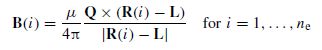
Figure 5.1 The magnetic field B at each electrode is calculated with respect to the moment of the dipole and the distance between the centre of the dipole and the electrode
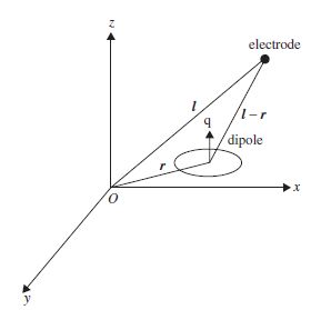
Figure 5.2 The magnetic field B at each electrode is calculated with respect to the accumulated moments of the m dipoles and the distance between the centre of the dipole volume and the electrode
where Q is the dipole moment, | . | denotes absolute value, and × represents the outer vector product. This is frequently used as the model for magnetoencephalographic (MEG) data observed by magnetometers. This can be extended to the effect of a volume containing m dipoles at each one of the ne electrodes (Figure 5.2).
In the m-dipole case the magnetic field at point j is obtained as
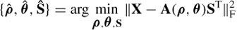
where ne is the number of electrodes and Lj represents the location of the j th dipole. The matrix B can be considered as B = [B(1), B(2), …, B(ne)]. On the other hand, the dipole moments can be factorized into the product of their unit orientation moments and strengths, i.e. B = GQ (normalized with respect to µ0/4π), where G = [ g( 1 ), g( 2), …, g(m)] is the propagating medium (mixing matrix) and Q = [Q1, Q2, …Q m ]T. The vector g(i) has the dimension 1 × 3 (thus G is m × 3). Therefore B = GMS. GM can be written as a function of location and orientation, such as H (L, M), and therefore B = H (L, M) S. The initial solution to this problem used a least-squares search that minimizes the difference between the estimated and the measured data:
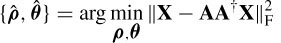
where X is the magnetic (potential) field over the electrodes. The parameters to be estimated are location, dipole orientation, and magnitude for each dipole. This is subject to knowing the number of sources (dipoles). If too few dipoles are selected then resulting parameters are influenced by the missing dipoles. On the other hand, if too many dipoles are selected the accuracy will decrease since some of them are not valid brain sources. Also, the computation cost is high due a number of parameters being optimized simultaneously. One way to overcome this is by converting this problem into a projection minimization problem as

The matrix  projects the data on to the orthogonal complement of the column space of H(L, M). X can be reformed by a singular value decomposition (SVD), i.e. X = U∑V T. Therefore
In this case orthogonal matrices preserve the Frobenius norm. The matrix Z = U∑ is m × m unlike X, which is under ne T, with T the number of samples. Generally, the rank of X satisfies rank(X) ≤ m, T >> m, and ∑ can have only m nonzero singular values. This means that the overall computation cost has been reduced by a large amount. The SVD can also be used to reduce the computation cost for  . The pseudoinverse H † can be decomposed as
  , where
  .
.
The dipole model, however, requires a priori knowledge about the number of sources, which is usually unknown.
Many experimental studies and clinical experiments have examined the developed source localization algorithms. Yao and Dewald [14] have evaluated different cortical source localization methods such as the moving dipole (MDP) method [15], the minimum Lp norm [16], and low-resolution tomography (LRT), as for LORETA (low-resolution electromagnetic tomography algorithm) [17] using simulated and experimental EEG data. In their study, only the scalp potentials have been taken into consideration.
In this study other source localization methods such as the cortical potential imaging method [18] and the three-dimensional resultant vector method [19] have not been included. These methods, however, follow similar steps to the minimum norm methods and dipole methods respectively.
5.2 Overview of the Traditional Approaches
5.2.1 ICA Method
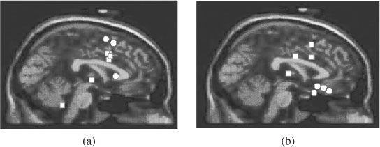
In a simple approach by Spyrou et al. [20] ICA is used to separate the EEG sources. The correlation values of the estimated sources and mixtures are then used to build up the model of the mixing medium. The LS approach is then used to find the sources using the inverse of these correlations, i.e. dij ≈ 1/(Cij)0.5, where dij shows the distance between source i and electrode j, and Cij shows the correlation of their signals. The method has been applied to separate and localize the sources of P3a and P3b subcomponents for five healthy subjects and five patients. A study of ERP components such as P300 and its constituent subcomponents is very important in analysis, diagnosing, and monitoring of mental and psychiatric disorders. Source location, amplitude, and latency of these components have to be quantified and used in the classification process. Figure 5.3 illustrates the results superimposed on two MRI templates for the above two cases. It can be seen that for healthy subjects the subcomponents are well apart whereas for schizophrenic patients they are geometrically mixed.
Figure 5.3 Localization results for (a) the schizophrenic patients and (b) the normal subjects. The circles represent P3a and the squares represent P3b
5.2.2 MUSIC Algorithm
Multiple signal classification (MUSIC) [21] has been used for localization of the magnetic dipoles within the brain [22–25] using EEG signals. In an early development of this algorithm a single-dipole model within a three-dimensional head volume is scanned and projections on to an estimated signal subspace are computed [26]. To locate the sources, the user must search the head volume for multiple local peaks in the projection metric. In an attempt to overcome the exhaustive search by the MUSIC algorithm a recursive MUSIC algorithm was developed [22]. Following this approach, the locations of the fixed, rotating, or synchronous dipole sources are automatically extracted through a recursive use of subspace estimation. This approach tries to solve the problem of how to choose the locations that give the best projection on to the signal (EEG) space. In the absence of noise and using a perfect head and sensors model, the forward model for the source at the correct location projects entirely into the signal subspace. In practice, however, there are estimation errors due to noise. In finding the solution to the above problem there are two assumptions that may not be always true: first, the data are corrupted by additive spatially white noise and, second, the data are produced by a set of asynchronous dipolar sources. These assumptions are waved in the proposed recursive MUSIC algorithm [22].
The original MUSIC algorithm for the estimation of brain sources may be described as follows. Consider the head model for transferring the dipole field to the electrodes to be A(ρ, θ), where ρ and θ are the dipole location and direction parameters respectively. The relationship between the observations (EEG), X, the model A, and the sources S is given as
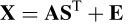
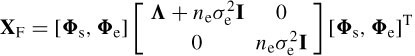
where E is the noise matrix. The goal is to estimate the parameters { ρ,θ, S }, given the data set X. The correlation matrix of X, i.e. Rx, can be decomposed as
or
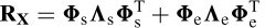
where Λs = Λ+ neσ2e I is the m × m diagonal matrix combining both the model and noise eigenvalues and Λe = ne σ 2e I is the (ne – m) × (ne – m) diagonal matrix of noiseonly eigenvalues. Therefore, the signal subspace span (Φs) and noise-only subspace span (Φe) are orthogonal. In practice, T samples of the data are used to estimate the above parameters, i.e.

where the first m left singular vectors of the decomposition are designated as  and the remaining eigenvectors as
  . Accordingly, the diagonal matrix
  contains the first m eigenvalues and
  contains the remainder. To estimate the above parameters the general rule using least-squares fitting is
where || . || F denotes the Frobenius norm. Optimal substitution [27] gives:
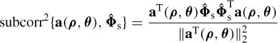
where A † is the Moore–Penrose pseudoinverse of A [28]. Given that the rank of A (ρ, θ) is m and the rank of  is at least m, the smallest subspace correlation value, Cm = subcorr{ A (ρ, θ),
  } m, represents the minimum subspace correlation (maximum principal angle) between principal vectors in the column space of A(ρ ,θ) and the signal subspace
  . In MUSIC, the subspace correlation of any individual column of A(ρ, θ) i.e. a(ρi, θi) with the signal subspace must therefore equal or exceed this minimum subspace correlation:

 approaches
  when the number of sample increases or the SNR becomes higher. Then the minimum correlation approaches unity when the correct parameter set is identified, such that the m distinct sets of parameters (ρi,θi) have subspace correlations approaching unity. Therefore a search strategy is followed to find the m peaks of the metric [22]
where  denotes the squared Euclidean norm. For a perfect estimation of the signal subspace m global maxima equal to unity are found. This requires searching for both sets of parameters ρ and θ. In a quasilinear approach [22] it is assumed that a(ρi, θi) = G (ρi, θi), where G (.) is called the gain matrix. Therefore, in the EEG source localization application, first the dipole parameters ρi that maximize the subcorr{ G (ρi),
  } are found and then the corresponding quasilinear θi that maximize this subspace correlation are extracted. This avoids explicitly searching for these quasilinear parameters, reducing the overall complexity of the nonlinear search. Therefore, the overall localization of the EEG sources using classic MUSIC can be summarized in the following steps:
 . Slightly overspecifying the rank has little effect on performance whereas underspecifying it can dramatically reduce the performance.
 }.
}. where C1 is the maximum subspace correlation. Locate m or fewer peaks in the grid. At each peak, refine the search grid to improve the location accuracy and check the second subspace correlation.
A large second subspace correlation is an indication of a rotating dipole [22]. Unfortunately, there are often errors in estimating the signal subspace and the correlations are computed at only a finite set of grid points. A recursive MUSIC algorithm overcomes this problem by recursively building up the independent topography model. In this model the number of dipoles is initially considered as one and the search is carried out to locate a single dipole. A second dipole is then added and the dipole point that maximizes the second subspace correlation, C2, is found. At this stage there is no need to recalculate C1. The number of dipoles is increased and the new subspace correlations are computed. If m topographies comprise m1 single-dipolar topographies and m2 two-dipolar topographies, then the recursive MUSIC will first extract the m1 single-dipolar models. At the (m1 + 1)th iteration, no single dipole location that correlates well with the subspace will be found. By increasing the number of dipole elements to two, the searches for both have to be carried out simultaneously such that the subspace correlation is maximized for Cm1 +1. The procedure continues to build the remaining m2 two-dipolar topographies. After finding each pair of dipoles that maximizes the appropriate subspace correlation, the corresponding correlations are also calculated.
Another extension of MUSIC-based source localization for diversely polarized sources, namely recursively applied and projected (RAP) MUSIC [24], uses each successively located source to form an intermediate array gain matrix (similar to the recursive MUSIC algorithm) and projects both the array manifold and the signal subspace estimate into its orthogonal complement. In this case the subspace is reduced. Then the MUSIC projection to find the next source is performed. This method was initially applied to localization of the magnetoencephalogram (MEG) [24,25].
In a recent study by Xu et al. [29], another approach to EEG three-dimensional (3D) dipole source localization using a nonrecursive subspace algorithm, called FINES, has been proposed. The approach employs projections on to a subspace spanned by a small set of particular vectors in the estimated noise-only subspace, instead of the entire estimated noise-only subspace in the case of classic MUSIC. The subspace spanned by this vector set is, in the sense of the principal angle, closest to the subspace spanned by the array manifold associated with a particular brain region. By incorporating knowledge of the array manifold in identifying the FINES vector sets in the estimated noise-only subspace for different brain regions, this approach is claimed to be able to estimate sources with enhanced accuracy and spatial resolution, thus enhancing the capability of resolving closely spaced sources and reducing estimation errors. The simulation results show that, compared to classic MUSIC, FINES has a better resolvability of two closely spaced dipolar sources and also a better estimation accuracy of source locations. In comparison with RAP MUSIC, the performance of FINES is also better for the cases studied when the noise level is high and/or correlations among dipole sources exist [29].
A method for using a generic head model, in the form of an anatomical atlas, has also been proposed to produce EEG source localizations [30]. The atlas is fitted to the subject by a nonrigid warp using a set of surface landmarks. The warped atlas is used to compute a finite element model (FEM) of the forward mapping or lead-fields between neural current generators and the EEG electrodes. These lead-fields are used to localize current sources from the EEG data of the subject and the sources are then mapped back to the anatomical atlas. This approach provides a mechanism for comparing source localizations across subjects in an atlas-based coordinate system.
5.2.3 LORETA Algorithm
The low-resolution electromagnetic tomography algorithm (LORETA) for localization of brain sources has already been commercialized. In this method, the electrode potentials and matrix X are considered to be related as

where S is the actual (current) source amplitudes (densities) and L is an ne × 3m matrix representing the forward transmission coefficients from each source to the array of sensors. L has also been referred to as the system response kernel or the lead-field matrix [31]. Each column of L contains the potentials observed at the electrodes when the source vector has unit amplitude at one location and orientation and is zero at all others. This requires the potentials to be measured linearly with respect to the source amplitudes based on the superposition principle. Generally, this is not true and therefore such assumption inherently creates some error. The fitted source amplitudes, Sn, can be roughly estimated using an exhaustive search through the inverse least-squares (LS) solution, i.e.
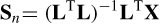
L may be approximated by 3m simulations of current flow in the head, which requires a solution to the well-known Poisson equation [32]:
where σ is the conductivity of the head volume (Ωm)‒1 and ρ is the source volume current density (A/m3). A finite element method (FEM) or boundary element method (BEM) is used to solve this equation. In such models the geometrical information about the brain layers and their conductivities [33] have to be known. Unless some a priori knowledge can be used in the formulation, the analytic model is ill-posed and a unique solution is hard to achieve.
On the other hand, the number of sources, m, is typically much larger than the number of sensors, ne, and the system in Equation (5.15) is underdetermined. Also, in the applications where more concentrated focal sources are to be estimated such methods fail. As will be seen later, using a minimum norm approach, a number of approaches choose the solution that satisfies some constraints, such as the smoothness of the inverse solution.
One approach is the minimum norm solution, which minimizes the norm of S under the constraint of the forward problem:

with a solution as
The motivation of the minimum norm solution is to create a sparse solution with zero contribution from most of the sources. This method has the serious drawback of poor localization performance in three-dimensional (3D) space. An extension to this method is the weighted minimum norm (WMN), which compensates for deep sources and hence performs better in 3D space. In this case the norms of the columns of L are normalized. Hence the constrained WMN is formulated as

with a solution as
where W is a diagonal 3m × 3m weighting matrix, which compensates for deep sources in the following way:
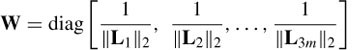
where || Li ||2 denotes the Euclidean norm of the ith column of L, i.e. W corresponds to the inverse of the distances between the sources and electrodes.
In another similar approach a smoothing Laplacian operator is employed. This operator produces a spatially smooth solution agreeing with the physiological assumption mentioned earlier. The function of interest is then

where B is the Laplacian operator. This minimum norm approach produces a smooth topography in which the peaks representing the source locations are accurately located.
An FEM has been used to achieve a more anatomically realistic volume conductor model of the head, in an approach called the adaptive standardized LORETA/FOCUSS (focal underdetermined system solver) (ALF) [34]. It is claimed that using this applicationspecific method a number of different resolution solutions using different mesh intensities can be combined to achieve the localization of the sources with less computational complexities. Initially, FEM is used to approximate solutions to (5.23) with a realistic representation of the conductor volume based on magnetic resonance (MR) images of the human head. The dipolar sources are presented using the approximate Laplace method [35].
5.2.4 FOCUSS Algorithm
The FOCUSS [34] algorithm is a high-resolution iterative WMN method that uses the information from the previous iterations as

where C = (Q‒1)T Q‒1 and Qi = WQi‒1 [diag(Si‒1(1) … Si ‒1(3m)] and the solution at iteration i becomes
The iterations will stop when there is no significant change in the estimation. The result of FOCUSS is highly dependent on the initialization of the algorithm. In practice, the algorithm converges close to the initialization point and may easily become stuck in some local minimum. A clever initialization of FOCUSS has been suggested to be the solution to LORETA [34].
5.2.5 Standardized LORETA
Another option, referred to as standardized LORETA (sLORETA), provides a unique solution to the inverse problem. It uses a different cost function, which is
Hence, sLORETA uses a zero-order Tikhonov–Phillips regularization [36,37], which provides a possible solution to the ill-posed inverse problems:

where si indicates the candidate sources and S are the actual sources. Ri is the resolution matrix defined as
The reconstruction of multiple sources performed by the final iteration of sLORETA is used as an initialization for the combined ALF and weighted minimum norm (WMN or FOCUSS) algorithms [35]. The number of sources is reduced each time and Equation (5.19) is modified to

L f indicates the final n × m lead-field returned by sLORETA. Wi is a diagonal 3 mf × 3 mf matrix, which is recursively refined based on the current density estimated by the previous step:

and the resolution matrix in (5.28) after each iteration changes to

Iterations are continued until the solution does not change significantly. In another approach by Liu et al. [38], called shrinking standard LORETA-FOCUSS (SSLOFO), sLORETA is used for initialization. It then uses the re-WMN of FOCUSS. During the process the localization results are further improved by involving the above standardization technique. However, FOCUSS normally creates an increasingly sparse solution during iteration. Therefore, it is better to eliminate the nodes with no source activities or recover those active nodes that might be discarded by mistake. The algorithm proposed in Reference [39] shrinks the source space after each iteration of FOCUSS, hence reducing the computational load [38]. For the algorithm not to get trapped in a local minimum a smoothing operation is performed. The overall SSLOFO is therefore summarized in the following steps [38,39]:
Stay updated, free articles. Join our Telegram channel

Full access? Get Clinical Tree


