Electrocardiography
Elena B. Sgarbossa
Galen Wagner
Historical Perspective
The first demonstration of the human cardiac activity was made during a congress of physiologists in London by Augustus Waller, who, in May 1887, published the first single-lead electrocardiogram (ECG) (1). Waller recorded the electrical activity of the heart from a chest lead with a capillary electrometer (a glass tube filled with mercury) (2). When the electrometer was placed on the body surface, the current was transmitted from the chest to the mercury column, which would expand or contract. This movement could be observed only through a microscope and needed to be projected onto photographic paper (Fig. 59.1).
The pioneer of clinical electrocardiography, however, was Willem Einthoven. Einthoven had a background in physics and mathematics (3). To refine Waller’s concept, Einthoven worked in his laboratory in the Netherlands for years, first with the electrometer and later with the string galvanometer (2). The galvanometer was an instrument developed in 1897 by Clément Ader for telegraphic transmissions. It reduced the distortion of the electrometer because it consisted of a thin wire extended between the poles of a magnet, but it still required the use of both a microscope and photographic paper. Einthoven presented his idea of applying the galvanometer to the recording of the cardiac electrical activity in 1903 (2). He also coined the term elektrokardiogramm in German (the dominant language at the time for scientific publications) and labeled the recorded waveforms P, Q, R, S, T, and U to differentiate them from the original, but incomplete, A, B, C, and D described by Waller. Einthoven also described numerous abnormal findings and created the bipolar limb lead system known as the Einthoven triangle (2).
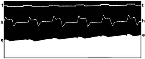 FIGURE 59.1. Reproduction of the first recording of an electrocardiogram by Waller. The electrical activity of the heart is recorded by movement on the surface of a mercury column (e). Chest wall movement is recorded by a mechanical lever (h). Time is indicated by t. (From Waller AD. A demonstration in man of electromotive changes accompanying the heart’s beat. J Physiol (Lond) 1887;8:229–234. ) |
This progress was observed skeptically by Waller, who, in 1911, expressed doubts on the clinical value of electrocardiography (4). The early electrocardiograph was extremely unwieldy. It required a continuous-flow water jacket for cooling the electromagnet. The camera and the optical system were an integral part of the apparatus, and an arc lamp projected the shadow of the string onto photographic paper. The electrodes were large bowls of saline solution in which the subject immersed his or her hands or feet. The machine occupied two rooms, and five people were required to operate it (5).
It was only after many years of these initial efforts that the ECG became regarded as a potentially useful tool in clinical practice (6). Several companies in Europe and in the United States initiated the commercial manufacturing of electrocardiographs. The first table-model electrocardiograph assembled in London was leased to Sir Thomas Lewis in 1911. Lewis worked intensively in recording both normal and abnormal cardiac activity. His work was pivotal in shifting the available knowledge from the laboratory to the clinical field. Keith and Flack had reported on the existence of the sinus node in 1907, and Lewis ascribed the origin of the cardiac impulse to it. He also proved the origin of ectopic tachycardias, studied atrial fibrillation, and introduced the concept of aberrant conduction. Lewis published several books, including the first textbook of electrocardiography (2).
During World War I, Lewis had a prominent disciple named Franklin Wilson, the youngest of a group of American cardiologists selected to work in England with him. At the end of the war, Wilson returned to the University of Michigan in Ann Arbor and obtained a string galvanometer. He worked with the galvanometer under the hospital stairwells, the only space appropriate for the large apparatus, which was smaller than the original model but still needed a wheeled trolley for transportation. Wilson’s investigations resulted in the theory of the ventricular gradient and in detailed descriptions of the bundle branch blocks (BBBs) (7). Perhaps Wilson’s best known contribution is his creation of a unipolar chest lead system connected to a central electrode (8).
By 1920, myocardial infarction had been recognized as an entity because of the reports by Herrick (9) and Pardee (10). In 1924, Einthoven was awarded the Nobel prize for his contribution, but the relevance of electrocardiography to clinical cardiology was not yet fully appreciated. Wilson himself published an article on heartbeat disorders in 1936 with no mention of electrocardiography (11).
Subsequent improvements to the original galvanometer led to further reduction in its size and to the current electronic technology. The first portable model was introduced in 1926, and
with it Lewis’ vision of electrocardiography as a standard diagnostic tool became a reality (3). At that time, two distinguished electrocardiographers and investigators, Langendorf and Pick, were attending medical school in Prague. Both physicians made their main scientific contributions later in the United States by perfecting the methodology of deductive reasoning for complex cardiac arrhythmias (12).
with it Lewis’ vision of electrocardiography as a standard diagnostic tool became a reality (3). At that time, two distinguished electrocardiographers and investigators, Langendorf and Pick, were attending medical school in Prague. Both physicians made their main scientific contributions later in the United States by perfecting the methodology of deductive reasoning for complex cardiac arrhythmias (12).
The “post-Wilson era” which began in the mid 1950s witnessed less radical, but yet important, developments in electrocardiography. By means of ingenious clinical-pathologic-correlations, investigators from different parts of the world elucidated the ECG manifestations of the many cardiac conditions. Outstanding contributors included the following: Lepeschkin, Surawicz, and Castellanos in the United States; Sodi-Pallares and Cabrera in Mexico; Rosenbaum in Argentina; Schamroth in South Africa; and Durrer and Wellens in the Netherlands. The introduction of invasive clinical electrophysiologic studies only confirmed in most cases the deductions of these pioneers (13).
In more recent years, emphasis in ECG research has shifted to the study of dynamic patterns inherent in certain parameters (especially ventricular repolarization) with the aid of the ambulatory recordings first introduced by Holter in 1961 and then by newer, potent digital storage and analysis techniques. The advent of effective myocardial reperfusion therapies has renewed the interest in the ECG manifestations of the acute ischemic syndromes. Finally, attempts at improving the resolution of standard electrocardiography have relied on an increase in the number of recording electrodes (body surface mapping) and on an improvement in the signal-to-noise ratio of the higher frequency signals by averaging and filtering (signal-averaged electrocardiography). Initial results with these techniques are promising, but their roles in clinical practice are still unclear.
Despite the development of more sophisticated and expensive cardiac diagnostic tests, the standard 12-lead ECG remains an integral part of the clinical evaluation of all cardiac patients, particularly those with ischemic heart disease or rhythm disturbances.
Anatomic References
The “view” of the electrical activity recorded from any surface ECG electrode is determined by the relative position of the heart. With the individual standing, the heart lies rather horizontally with the atria at its base and the ventricles at its apex (14). Because the heart is a conical structure rotated over its long axis, the right atrium and ventricle are more anterior than the left chambers, and the right and left sides of the heart are not aligned with the homonymous sides of the body. Thus, the interventricular septum is almost parallel to the frontal, not the sagittal, plane, and the left ventricular (LV) free wall (usually considered a lateral structure) includes nearly 300 degrees of the LV circumference and faces superiorly, posteriorly, and inferiorly (5).
Electrocardiographic Recording
The 1 Leads
The cardiac electrical activity is recorded through 12 surface leads named I, II, III, aVR, aVL, aVF, V1, V2, V3, V4, V5, and V6. The first six points are recorded with electrodes located on the limbs, whereas leads V1 to V6 are recorded from the chest (Fig. 59.2).
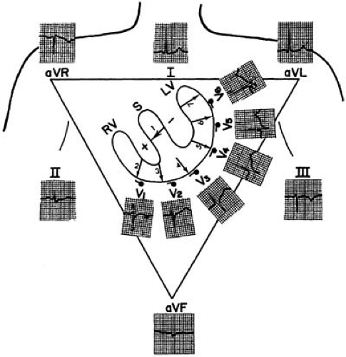 FIGURE 59.2. The standard 12 leads are shown with their recording sites. Both the frontal and the horizontal planes are depicted. Vectors 1 to 7 show the normal sequence of activation of the septum (S) and ventricles from the horizontal plane. LV, left ventricle; RV, right ventricle. (From Gazes PC, ed. Clinical cardiology: a bedside approach. Chicago: Year Book, 1983:39. ) |
Leads I, II, and III were first used when Einthoven placed recording electrodes on both arms and the left leg, to form an equilateral triangle. An additional electrode on the right leg was used for grounding. Leads I to III are bipolar because they record potential differences between two electrodes. For lead I, the left arm electrode is the positive pole, and the right arm electrode is the negative pole. Lead II has its positive pole on the left leg and its negative pole on the right arm, and it provides a view of the electrical activity along the long axis of the heart. Lead III has its positive pole on the left leg and its negative pole on the left arm. Between leads I, II, and III are 60-degree angles. These wide viewing gaps are filled with the augmented unipolar (“aV”) leads aVR, aVL, and aVF, which record the electrical activity between the exploring limb electrode and a reference created connecting the other two limb electrodes together trough a 5000-ohm resistor (the Wilson central terminal) (15). Lead aVF, for example, measures the potential difference between the left leg and the average of the potentials at the right and left arms. The addition of these three aV leads to the triaxial reference system produces an hexaxial system, with the six leads separated by angles of only 30 degrees. The gap between leads II and II is filled by lead aVR, that between leads II and III by lead aVF, and that between leads III and I, by lead aVL. This provides a perspective of the frontal plane, as illustrated in Figure 59.2. The limb leads are presented in the order I, II, II, aVR, aVL, and aVF, which spatially correspond to 0, 60, 120, -150, -30, and 90 degrees, respectively.
The last set of leads introduced to clinical practice were the six unipolar precordial leads (V1 to V6) (3). Augmentation is not necessary because the recording electrodes are close to the heart. The Wilson central terminal provides their negative poles, whereas the sites of the exploring electrode are determined by bony landmarks on the anterior and left lateral aspects of the precordium (Table 59.1 and Fig. 59.3). The angles between these leads are slightly smaller than those between the
six frontal plane leads. Lead V1 is located where the extension of the heart short axis (i.e., a perpendicular to the interatrial and interventricular septa) intersects with the precordial body surface. Because V1 provides a right anterior to left posterior view, it distinguishes better between left and right cardiac electrical activity than does a lead providing a right lateral to left lateral view (e.g., lead I).
six frontal plane leads. Lead V1 is located where the extension of the heart short axis (i.e., a perpendicular to the interatrial and interventricular septa) intersects with the precordial body surface. Because V1 provides a right anterior to left posterior view, it distinguishes better between left and right cardiac electrical activity than does a lead providing a right lateral to left lateral view (e.g., lead I).
TABLE 59.1 Placement of precordial lead electrodes | ||||||||||||||||||||||||||||
|---|---|---|---|---|---|---|---|---|---|---|---|---|---|---|---|---|---|---|---|---|---|---|---|---|---|---|---|---|
| ||||||||||||||||||||||||||||
Limitations of the Current 12-Lead System
Poor Orthogonality and Redundancy
A set of three ECG leads is orthogonal if their lead vectors are at 90-degree angles with each other, thus permitting the accurate detection of the onset and offset of ECG waveforms in all spatial directions. Orthogonality in the current 12-lead system is meager because the sagittal and anteroposterior components of cardiac activity are recorded poorly by the limb leads, whereas the precordial leads miss the vertical components. Also, the current 12-lead system provides for superfluous recording points. Of the standard ECG, probably only eight components capture independent information on cardiac electrical activity.
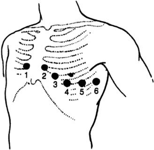 FIGURE 59.3. Location of the precordial lead electrodes. (From The electrocardiogram: fundamentals. In: Goldschlager N, Goldman MJ, eds. Principles of clinical electrocardiography. Stamford, CT: Appleton & Lange, 1989:1–10. ) |
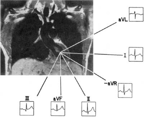 FIGURE 59.4. The panoramic display of the 12-lead electrocardiogram in an ideal sequential spatial order. (From Anderson ST, Pahlm O, Selvester RH, et al. Panoramic display of the orderly sequenced 12-lead ECG. J Electrocardiol 1994;27:347–352. ) |
Inappropriate Lead Sequencing and Gap in the Frontal Plane
In the ECG, the precordial leads are displayed to depict an orderly progression in the horizontal plane. Leads V1 to V6 faithfully show the spatial sequence of electrical activation (from the basal right ventricle to the midposterior LV wall). The limb leads, instead, depict a disordered spatial sequence. Leads I, II, II, aVR, aVL, and aVF correspond spatially to 0, 60, 120, -150, -30, and 90 degrees, respectively. Such array has been consecrated by usage, but it is counterintuitive. If an analogous distribution were selected for the horizontal plane, the precordial leads would be reordered as V2, V4, V6, -V3, V1, and V5 (16). This would considerably compromise the ability of the interpreter to understand the electrical phenomena in that plane rapidly. A more logical sequencing for the limb leads would be aVL, I, -aVR, II, aVF, and III (or -30, 0, 30, 60, 90, and 120 degrees); the inclusion of a negative aVR would allow to record ECG phenomena at 30° (Fig. 59.4).
Special Leads
Some leads are not considered part of the standard ECG but are useful in specific circumstances. Posterior leads (V7, V8, and V9) increase the ECG sensitivity for injury in the posterior wall (17) (Table 59.1). Right precordial leads (V3R, V4R) are particularly useful for the diagnosis of right ventricular infarcts and of some congenital abnormalities (Table 59.1) (18). A routine use of the negative aVR (at 30 degrees) would add useful information to the standard ECG, and it would be less likely to be overlooked during routine ECG interpretation (19,20,21).
The P wave is not always distinctly seen in the 12-lead ECG, but it may be easily identified with special leads. Distinct P waveforms can be seen by placing the right and left arm leads in various chest positions (if possible, parallel to the vector of atrial depolarization) while recording lead I (the Lewis lead). Atrial activity can also be recorded semiinvasively from leads
placed in the esophagus because the anterior wall of the esophagus lies against the left atrium. In patients with dual-chamber pacemakers, atrial electrograms can be recorded by telemetry from the pacing electrodes. In patients recovering from cardiac surgery, the placement of temporary epicardial pacing electrodes allows the direct recording of atrial activity.
placed in the esophagus because the anterior wall of the esophagus lies against the left atrium. In patients with dual-chamber pacemakers, atrial electrograms can be recorded by telemetry from the pacing electrodes. In patients recovering from cardiac surgery, the placement of temporary epicardial pacing electrodes allows the direct recording of atrial activity.
Equipment
Electrocardiographers are calibrated to give a deflection of 10 mm/mV (this calibration is seen at the beginning or end of the ECG). ECG paper is graph paper divided in little squares of 1 mm each and bigger squares of 5 mm each. The paper speed is standardized to 25 mm/second. One mm equals 0.1 mV.
Commercial systems provide ECG programs with stereotyped methodologies of measurement. The only limb ECG leads that digital electrocardiographs record are leads I and II; the remaining limb leads are calculated in real time based on the Einthoven law (I + III = II) and using relationships derived from lead vectors for the aV leads. For the calculation of the electrical QRS axis, the entire QRS complex area is used. This is an advantage over the manual QRS axis estimation, based mainly on R-wave measurements.
Current electrocardiographs use digital technology. Analog data are converted into digital signals that are later processed (22). The use of compression techniques allows storage and subsequent retrieval of serial ECG recordings, as well as remote transmission of ECG data, for example, to hand-held computers for “real-time” interpretation by a cardiologist (23). After digital transmission or retrieval of serial measurements, output data can be compared with input data.
Basic Principles
Membrane Properties, Action Potential, and Cardiac Activation
Myocytes maintain a potential difference between the cell interior and exterior of approximately -90 mV. This electrical transmembrane gradient depends on the chemical transmembrane gradient, which exists because the concentration of negative ions is higher inside the cell than outside. Such uneven distribution of ions and their flow in and out of the cell is regulated by channels, which are complex molecular structures housed in the cell membrane (24). Electric stimuli change the resting potential inside the cell from -90 mV to about +30 mV (depolarization), and this electrical activity is the action potential. Depolarization initiates the propagation of the impulse along both the inner and outer sides of the “polarized” membrane. Thus, the electrical front, which can be represented as a vector, flows from the positively (depolarized) to the negatively (resting) charged cells. The earliest ventricular activation occurs in the left side of the septum. Then the depolarization front reaches the septum right side and the anterior wall, thus following an inside-out course. The action potential shapes differ considerably between endocardial and epicardial myocytes, secondary to differences in the distribution of currents (and channel proteins) among cardiac layers (25).
The phenomenon underlying depolarization at the cellular level is the inflow of the positive ions sodium and calcium. This inward current is at some point exceeded by an outward current of potassium ions, which ends the electrical systole and leads to repolarization (i.e., restitution of membrane polarity). In the atrium, repolarization proceeds in the same direction as atrial depolarization, and thus the polarity of the repolarization waveform is opposite that of depolarization. Ventricular repolarization, however, follows an inverted path. It travels from epicardium to endocardium; therefore, the repolarization waveform polarity is the same as that of depolarization. This behavior is the basis for the concept of ventricular gradient. The ventricular gradient measures the magnitude of the integral between the QRS complex and the T wave (i.e., between depolarization and repolarization). If all ventricular action potentials had the same magnitude and duration, the ventricular gradient would be zero. Yet repolarization forces start and end at different times within the various ventricular areas, and they also differ in duration (slope of phase 3 of the action potential). Thus, within the ventricles there is both spatial and temporal variability, or repolarization dispersion (26). To this dispersion may also contribute an additional population of cardiac cells, the intramural “M cells” (10).
Cardiac Activation: Impulse Formation, and Conduction
The heart can be considered as a dipole with a positive and a negative charge. At any given time, cardiac cells are in various stages of activation (i.e., depolarization and repolarization). The formation (i.e., pacemaking) and timely conduction of an electrical impulse depend on cardiac cells that are strategically placed and arranged in nodes, bundles, and an intraventricular network that end in Purkinje cells. All these specialized cells lack contractile capability, but they can act as pacemakers (i.e., spontaneously generate electrical impulses) and alter conduction speed. The intrinsic pacemaking rate is fastest in the sinus node, located in the right atrium, and is slowest in the Purkinje cells.
The intraventricular conduction network includes the common bundle of His and its right and left bundle branches, which extend along the septum toward their respective ventricles. The left bundle branch is a diffuse structure that fans broadly over the septum toward the two mitral valve papillary muscles. In the left bundle branch, two divisions can usually be distinguished; they are called anterior and posterior but are indeed superior and inferior, respectively. Because the right bundle branch remains compact until it reaches the distal interventricular septal surface (where it branches into the septum and toward the lateral right ventricular wall), many authors consider the intraventricular conduction system to be trifascicular (27,28). These intraventricular conduction pathways are composed of Purkinje cells with both pacemaking and rapid impulse conduction capabilities. Purkinje fibers branch into networks that extend just beneath the endocardial surface.
The normal activation sequence begins at the midseptum, continues in the epicardial right ventricular wall near the apex, then at the lateral and basal LV, and ends at the basal septum (Fig. 59.5). The wavefront departs from the sinus node and travels through the right and left atria in a centrifugal manner. On arrival at the atrioventricular (AV) node, the impulse is delayed, allowing for a sequential, rather than simultaneous, contraction of the ventricles after the atria. Because the Purkinje system provides a specialized path for rapid activation, the entire ventricular mass can be depolarized in a short time (similar to the depolarization timing of the much smaller atria). The impulses then proceed slowly from endocardium to epicardium throughout both ventricles (29).
Electrical Bases for Electrocardiography and Vectorcardiography
Differences in cardiac potentials of a single cardiac cell or a small group of cells do not produce enough current to be
detected on the body surface. Electrical representation on the ECG depends on the activation of most of the atrial and ventricular masses. The depolarization process produces a relatively high-frequency ECG waveform. The earliest QRS complex is recorded in right precordial leads. While depolarization persists, the ECG recording returns to baseline. Repolarization is then represented by the ST segment and the T and U waves (10). Once the cells are in their resting state, the ECG records a flat baseline.
detected on the body surface. Electrical representation on the ECG depends on the activation of most of the atrial and ventricular masses. The depolarization process produces a relatively high-frequency ECG waveform. The earliest QRS complex is recorded in right precordial leads. While depolarization persists, the ECG recording returns to baseline. Repolarization is then represented by the ST segment and the T and U waves (10). Once the cells are in their resting state, the ECG records a flat baseline.
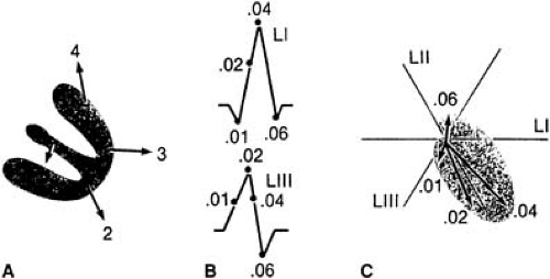 FIGURE 59.5. Correlation between the order of ventricular activation (A), scalar electrocardiogram (B), and vectorcardiogram (C). A: The sequence of ventricular activation is represented by four instantaneous frontal plane vectors. B: The four vectors plotted on leads I and III at the appropriate time during inscription of the QRS complex. C: Each of the four vectors is derived in the frontal plane. A line joining the ends of the vectors results in a frontal plane QRS loop. L, lead. (From Fisch C. Electrocardiography and vectorcardiography. In: Braunwald E, ed. Heart disease: a textbook of cardiovascular medicine, 4th ed. Philadelphia: WB Saunders, 1992:116–160. ) |
On the 12-lead ECG, only 10% to 15% of the ventricular activation process can be seen; the remaining activation forces cancel each other. The normal right ventricle has no ECG representation because its forces are obscured by the dipoles generated in the massive LV. The summation of all cardiac electrical forces can be represented with a single vector that originates at the center of the Einthoven triangle and whose arrowhead points to the positive pole. If all instantaneous single vectors were plotted consecutively, a vector loop would be formed in each of the three spatial planes (frontal, sagittal, and horizontal). Such recording constitutes a vectorcardiogram (Fig. 59.5). The vectorcardiogram integrates two surface leads out of three (named X, Y, and Z) in an orthogonal system and depicts a separate loop for each of the ECG components (P wave, QRS complex, T wave, and U wave). The vectorcardiogram is superior to the ECG in that it provides information not only on magnitude and direction (i.e., positive or negative) of the signals, but also on spatial orientation.
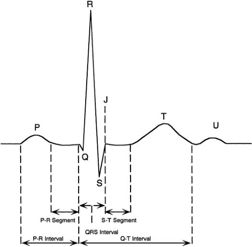 FIGURE 59.6. Waveforms and intervals of the electrocardiogram. (From Wagner GS, ed. Marriott’s practical electrocardiography, 9th ed. Baltimore: Williams & Wilkins, 1994:13. ) |
Normal Electrocardiographic Waveforms
Overview
The waves on the ECG represent a coincident voltage gradient generated by cellular electrical activity within the heart. The normal waveforms are depicted in Figure 59.6. The origin of the cardiac impulse in the sinus node is electrocardiographically mute; the initial recordable wave for each cardiac cycle is the P wave, which represents the spread of activation through the atria. Ventricular activation results in the QRS complex, which may appear as one (monophasic), two (diphasic), or three (triphasic) individual waveforms. Low-amplitude or narrow waves are denoted by lowercase letters (e.g., q wave) and taller, wider waves are denoted by capital letters (e.g., Q wave).
The T wave represents ventricular recovery and is sometimes followed by a small upright deflection, the U wave. The ST segment is the interval between the end of ventricular activation (the plateau phase of the action potential) and the beginning of ventricular recovery. The QT interval measures the time from ventricular activation onset to end of ventricular recovery. At low heart rates the PR, ST, and TP segments are at the same horizontal level (i.e., the isoelectric line), considered the baseline for measuring various waveform amplitudes (30).
The T wave represents ventricular recovery and is sometimes followed by a small upright deflection, the U wave. The ST segment is the interval between the end of ventricular activation (the plateau phase of the action potential) and the beginning of ventricular recovery. The QT interval measures the time from ventricular activation onset to end of ventricular recovery. At low heart rates the PR, ST, and TP segments are at the same horizontal level (i.e., the isoelectric line), considered the baseline for measuring various waveform amplitudes (30).
P Wave
The first part of the P wave represents the activation in the right atrium, and the middle and final sections of the P wave are recorded during left atrial activation. The normal P wave is rounded and upright in leads I and II and from V2 to V6. Its maximum amplitude is 0.25 mV in lead II (or 25% of the R wave), and its duration is 0.08 second. The P-wave axis is approximately 60 degrees. The intrathoracic position of the right and left atria determines that the activation front be directed first anteriorly, then posteriorly. The right atrium faces lead V1, in which the initial portion of the P wave appears positive while its terminal part appears negative.
Ta Segment
The Ta segment (or Ta wave) represents atrial repolarization and may be seen in physiologically normal individuals, but it is more often obscured by the QRS complex and the early part of the ST segment. The Ta wave direction is opposite that of the P wave. A normal but prominent Ta wave may produce PR segment depression and mimic a pathologic Q wave.
PR Interval
The time from onset of the P wave to onset of the QRS complex (whether its first wave is a Q or an R wave) is the PR interval. It encompasses the time between the onset of atrial depolarization in the myocardium adjacent to the sinus node and the onset of ventricular depolarization in the myocardium adjacent to the Purkinje network. A major portion of it is inscribed during the slow conduction through the AV node. The normal PR interval measures 0.12 to 0.22 second. The PR interval increases with age. It shortens as heart rates increases; this effect depends on higher sympathetic and lower vagal tones. Incremental atrial pacing at rest, however, prolongs the PR interval. The time from the end of the P wave to the onset of the QRS complex is called PR segment.
QRS Complex
The QRS complex represents ventricular activation. The contour of the QRS complex is peaked because it is composed of high-frequency signals (Fig. 59.6). The normal ventricular activation can be summarized in four vectors (Fig. 59.5): (a) initial septal activation from left to right and anteriorly (inferiorly or superiorly), producing a positive deflection (R wave) at right recording sites; (b) an overlapping wave of excitation involving both ventricles, with the vector directed inferiorly and slightly to the left, which inscribes the midportion of the QRS complex; (c) unopposed activation of the apical and central portions of the LV and of the right ventricle with a resultant vector oriented posteriorly, inferiorly, and to the left; the posteriorly positioned LV is much thicker, and its activation predominates over that of the more anterior right ventricle, with a resulting negative deflection (i.e., S wave) in aVR and in right precordial leads and in an R wave in leads I, II, III, aVL, and left precordial leads; and (d) activation of the posterior basal portion of the LV and septum with a vector directed superiorly and posteriorly, which completes the S wave in V5 and V6.
The QRS complex measures 0.07 to 0.10 second and increases with the subject’s height (31). The QRS complex is measured from the beginning of the first appearing Q or R wave to the end of the last appearing R, S, or R′ wave. It tends to be slightly longer in male patients. The onset of the QRS complex is not recorded simultaneously in all ECG leads; this has implications when measuring QRS duration. The earliest QRS onset is recorded in right precordial leads (12). Computerized QRS measurements have the advantage of integrating information from the 12 leads.
Q Waves
A Q wave is a negative deflection at the onset of the QRS complex. It indicates that the net direction of early ventricular depolarization forces is oriented away from the positive axis of the recording lead at least by 90 degrees. Normal septal activation results in a rapid q wave in leads I, II, III, aVL, V5, and V6. The presence of Q waves in V1, V2, and V3 or the absence of small q waves in V5 and V6 is abnormal (13). Positional factors may also result in the inscription of prominent but narrow Q waves. If the septal vector is horizontal, Q waves may appear in lead aVF; if the electrical axis is vertical, Q waves may appear in aVL. Precordial lead electrodes misplaced in a high position may determine the inscription of Q waves and a pseudoinfarction pattern. In right precordial leads, qr and qS complexes may be normal (32).
R Waves
The first positive wave of the QRS complex is the R wave, regardless of whether it is preceded by a Q wave. The second activation vector results in an R wave in leads II and III, and the third vector produces an R wave in leads I, II, III, aVL, aVF, V5, and V6. The precordial leads provide a panoramic view of the cardiac electrical activity progressing from the right ventricle to the thicker LV; consequently, the R wave increases its amplitude and duration from V1 to V4 or V5. An rS pattern in leads V3R and V4R is normal. The R wave amplitude in V5 and V6 varies directly with LV dimension during exercise and with positional changes. Reversal of the normal sequence with larger R waves in V1 and V2 can be produced by right ventricular enlargement. When a second positive deflection occurs in any lead, it is called R′.
S Waves
A negative deflection following an R wave is an S wave. The third vector produces an S wave in leads aVr, V1, V2, V3, and occasionally, V4. The S wave in the precordial leads is large in V1, larger in V2, and then progressively smaller from V3 through V6. This sequence could be altered by ventricular enlargement. The last vector, directed superiorly and posteriorly, may result in a terminal S wave in leads I, V5, and V6. Leads V4R and V3R show an rS morphology in 80% of normal subjects (16).
Intrinsicoid Deflection
The time from the beginning of ventricular activation (onset of the QRS complex) to the point in which the impulse arrives
under a particular electrode is called the ventricular activation time. The downward deflection that follows is the intrinsicoid deflection. By definition, the intrinsicoid deflection can be measured only in precordial leads, but some authors applied this name to the turning point of the cardiac vector along the lead axis for the limb leads as well. For practical purposes, the estimate of the intrinsicoid deflection is the R peak time. It is measured from the onset of the QRS complex to the peak of the R wave or R′ wave. The R peak time is ≤0.04 second in V1 and V2, and ≤0.05 in V5 and V6 (33).
under a particular electrode is called the ventricular activation time. The downward deflection that follows is the intrinsicoid deflection. By definition, the intrinsicoid deflection can be measured only in precordial leads, but some authors applied this name to the turning point of the cardiac vector along the lead axis for the limb leads as well. For practical purposes, the estimate of the intrinsicoid deflection is the R peak time. It is measured from the onset of the QRS complex to the peak of the R wave or R′ wave. The R peak time is ≤0.04 second in V1 and V2, and ≤0.05 in V5 and V6 (33).
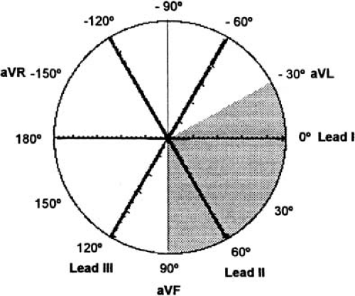 FIGURE 59.7. Frontal plane hexaxial reference system. The normal QRS axis in adults lies between –30 and +90 degrees (area in gray). |
QRS Axis
The QRS axis can be manually determined in the frontal plane in three steps: (a) the lead with the equiphasic deflection (defined as positive and negative components of the QRS complex of similar amplitudes) is identified; (b) the lead that is perpendicular to the initial lead is identified; and (c) if in this second lead the predominant QRS polarity is positive, the axis is equal to the positive pole of this lead; if the polarity is negative, the axis is equal to the negative pole of this lead. The normal electrical axis measures between –30 and + 90 degrees (Fig. 59.7). QRS axes between 0 and –30 degrees are considered “left axis deviation.”
The normal QRS complex is predominately positive in both leads I (with its positive pole at 0 degrees) and II (with its positive pole at +60 degrees). If the QRS is positive in lead I but negative in II, the axis is deviated leftward between –30 and –120 degrees. If the QRS is negative in I but positive in II, the axis is deviated rightward between +90 and ±180 degrees. The axis opposite to normal (with a predominately negative QRS orientation in both leads I and II) is rare.
The normal QRS axis is rightward in the neonate, moves during childhood to a vertical position, and then gradually moves through adulthood to a more horizontal position. In physiologically normal adults, the electrical axis is almost parallel to lead II, but it is more vertical in slender individuals and more horizontal in heavy individuals.
Because the cardiac base is firmly attached to the intrathoracic structures, true (i.e., anatomic) rotation of the heart on its long axis is limited to superior or inferior shifts of the relatively mobile cardiac apex. Most QRS axis deviations observed in the ECG in ventricular hypertrophies or fascicular blocks rather correspond to changes in the balance of epicardial versus endocardial activation forces or to different routes taken by the activation forces.
J Wave
The J wave (or Osborn wave) is a deflection that may appear on the ECG following the QRS complex as a result of electrical heterogeneities among the myocardial layers. It may be present in healthy patients with the early repolarization pattern (34).
ST Segment
The ST segment represents the time period in which the ventricular myocardium remains depolarized. The term ST segment is used whether the QRS complex ends in an R wave or in an S wave. At its junction with the QRS (i.e., J point), the ST segment forms a nearly 90-degree angle and then proceeds horizontally until it curves gently into the T wave. Slight upsloping (particularly in leads V1 to V3, and in V4R–V3R), downsloping, or horizontal depression of the ST segment may occur as a normal variant. The ST-segment length and appearance are influenced by factors that alter the duration of ventricular activation, such as exercise and BBB.
T Wave
The T wave represents exclusively uncanceled potential differences of ventricular repolarization (i.e., both spatial and temporal dispersion of repolarization) among the epicardium, M cells, and endocardium. The T wave accounts for 8% or less of the total time-voltage product of the heart (35). The T wave has a rounded but asymmetric shape, with the initial deflection longer than the terminal deflection. The peak of the T wave marks repolarization completion of the epicardial cells. The end of the T wave is temporally aligned with repolarization of the M cells (18). The M-cell repolarization is outlasted by that of the Purkinje cells, itself unlikely to generate an ECG wave.
The T-wave amplitude does not normally exceed 0.5 mV in limb leads or 0.10 mV in precordial leads. The T-wave vector and polarity are concordant with the R-wave vector. The T wave is always positive in lead I, nearly always positive or isoelectric in lead II, and may have any polarity in leads III and aVF (9). In precordial leads, the T wave is usually upright.
U Wave
When present, the U wave is a small, rounded wave following the T wave. It is most prominent in leads V2 to V3 and it usually shows the same direction as its preceding T wave, but in some patients it may be discordant (36). The U wave results from the last repolarization components. It may be generated by repolarization of the Purkinje network or by repolarization of the M cells (18,37,38).
QT Interval
The QT interval measures the time from the beginning of the QRS complex until the end of the T wave. It estimates the duration of both ventricular depolarization and repolarization, but it is used mainly as an estimate of ventricular recovery time. The term QT is used whether the QRS complex begins with a Q or an R wave.
Accurate QT measurements are elusive. One reason is that on a given ECG, the end of the T wave is not always obvious; its terminal portion may be isoelectric or merge with a U wave. This partially explains why the precise duration of the QT interval is notoriously difficult to determine, even by cardiologists, and to standardize (39). The problem has not been satisfactorily solved by automated programs, because of technical factors regarding acquisition of digital ECG signals.
The duration of the QT interval is affected by numerous physiologic variables. These include autonomic influences, circadian rhythms, electrolytes, and hormones. For example, the JT interval (i.e., the interval between the J point and the end of the T wave) is significantly shorter in men than in women (262±31 milliseconds versus 316±31 milliseconds), probably because repolarization is modulated by testosterone (40). Repolarization and the QT interval are also affected by drugs, an important reason to monitor QT-interval duration.
Another main factor influencing the QT interval is heart rate. Between the QT and the RR intervals is an inverse relationship that is nonlinear: as the heart rate increases, the QT interval initially shortens markedly and then shortens more gradually. Thus, QT-interval values require adjustment. The normal QT-interval values for a given heart rate are determined with mathematic formulas that estimate the corrected QT interval (QTc). Of the several QT correction formulas, that of Bazett (QTc = QT/VRR) is the most widely used. The normal value of QTc is up to 0.39 second in men and 0.44 second in women. Yet with the Bazett formula, the QTc remains undercorrected (i.e., artificially shortened) during bradycardia, whereas it paradoxically lengthens at faster rates (41). Alternative formulas to model the relationship between the RR and the QT intervals have improved the prediction of the QTc. Their adoption as part of standardization efforts at the clinical level, however, has not succeeded (42,43).
Expert guidelines for QT-interval measurement recommend measuring it manually in the lead where it is best viewed, averaging the QT-interval duration over three to five beats, and correcting the QT interval for heart rate. The best QT-interval correction formula, however, remains unclear, because none has been prospectively validated (44,45). Ethnic differences in the QT interval have not been demonstrated (46).
Normal Electrocardiographic Variants
ECGs as screening tests are requested worldwide daily for a number of purposes. A normal ECG is a good predictor of normal LV function, and it greatly reduces the need to request an echocardiogram to assess systolic function (47).
RSR′ Pattern in Lead V1
An RSR′ (or rSr′) pattern in lead V1 with a QRS duration less than 0.12 second is present in 2.4% of physiologically normal persons. The R′ wave may correspond to relatively late activation of the crista supraventricularis (48). In certain patients, an rSr′ complex in V1 may be a manifestation of a left-sided accessory pathway.
S1S2S3 Pattern
The S1S2S3 pattern has been observed in 20% of healthy subjects. The S waves in standard leads are inscribed when the terminal vector of the QRS complex originates in the outflow tract of the right ventricle or in the posterobasal septum and is directed rightward and superiorly. The typical S1S2S3 pattern (with all S waves larger than their preceding R waves) is not as common as the case wherein the amplitude of the S wave in lead I is smaller than that of the R wave.
Male Pattern and Early Repolarization
In men, ST-segment elevation of 1 to 3 mm in one or more precordial leads (typically including V2) is normal. It is called male pattern, and its prevalence decreases with age (49). Precordial ST-segment elevation is found instead only in 20% of healthy women, with no age variation.
Some healthy young men (particularly African Americans) have, in leads V1 to V3, ST-segment elevation up to 4 mm mimicking acute myocardial infarction or pericarditis (50,51) (Fig. 59.8). This pattern is called early repolarization. However, a premature ventricular recovery has not been demonstrated; the pattern could represent a mild intraventricular conduction delay in the right ventricle. Early repolarization appears to be an independent marker of enhanced aerobic condition (52).
Brugada Syndrome
An ECG pattern similar to that of early repolarization, the Brugada sign, consists of a right BBB (RBBB)–like pattern and coved ST-segment elevation in right precordial or inferior leads. The Brugada syndrome seems to be an ion channel disease similar to the long QT syndrome, inherited by an autosomal dominant pattern with variable penetrance (53,54) (Fig. 59.9). It is associated with ventricular tachyarrhythmias and sudden death (55).
The Brugada syndrome and early repolarization may have a common pathophysiologic basis (56). In both entities, ST-segment elevation is influenced by heart rate and autonomic tone.
Unusual T Waves
Negative T waves, particularly in precordial leads (from V6R to V2, and sometimes through V6) may be seen among young, usually African American, vagotonic persons. These T waves may show intermittent changes in polarity, and in some cases they follow an elevated ST segment (early repolarization syndrome). Transient inverted T waves have been documented in physiologically normal subjects after meals or after drinking cold water (57). Bifid T waves (i.e., T waves with two peaks different from a U wave) are present in 20% of children; their incidence decreases with age. A likely mechanism producing bifid T waves is a delayed right ventricular repolarization; an asynchronous repolarization of the anterior and posterior walls would inscribe two separate peaks in the T wave.
Approach to Electrocardiographic Diagnosis
Sensitivity, Specificity, and Predictive Accuracy
The ECG is a highly valuable diagnostic tool. ECG diagnoses, however, are made by inference and are therefore subject to error (58). To maximize the benefits from ECG information,
it is essential to apply the principles of prevalence, sensitivity, specificity, and predictive accuracy. The presence of a sign for a disorder is less informative in a clinically healthy population with a low prevalence of the disorder (59). Disorder prevalences between 40% and 60% result in the maximum drop or rise from pretest to posttest probability (60). Sensitivity represents the number of persons with a condition who do have a target ECG sign. A sign with perfect sensitivity will be positive in all patients with the condition; the absence of the sign rules out the condition. Specificity refers to the number of persons without a condition who do not have the target ECG sign. A sign with perfect specificity will be negative in all people without the condition; the presence of the sign makes a positive diagnosis. Sensitivity and specificity, however, depend on the spectrum of disease in the studied population.
it is essential to apply the principles of prevalence, sensitivity, specificity, and predictive accuracy. The presence of a sign for a disorder is less informative in a clinically healthy population with a low prevalence of the disorder (59). Disorder prevalences between 40% and 60% result in the maximum drop or rise from pretest to posttest probability (60). Sensitivity represents the number of persons with a condition who do have a target ECG sign. A sign with perfect sensitivity will be positive in all patients with the condition; the absence of the sign rules out the condition. Specificity refers to the number of persons without a condition who do not have the target ECG sign. A sign with perfect specificity will be negative in all people without the condition; the presence of the sign makes a positive diagnosis. Sensitivity and specificity, however, depend on the spectrum of disease in the studied population.
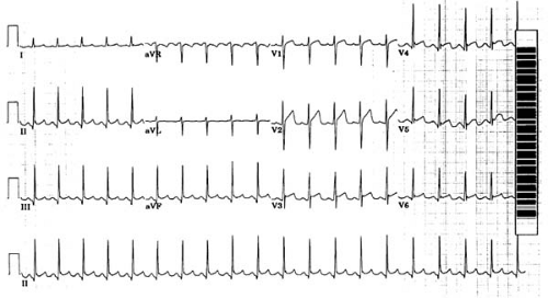 FIGURE 59.8. Electrocardiogram of patient with early repolarization and sinus tachycardia (19-year-old African American woman). ST-segment elevation is present in both inferior and precordial leads. |
At the time of requesting an ECG—when it is not known whether a particular disorder is present—a most helpful concept is that of predictive value. The positive predictive value is the proportion of patients with positive test results who have the condition. The negative predictive value is the proportion of patients with negative results who do not have the condition. Predictive values are clinically useful because they incorporate information on both the test (i.e., the ECG) and the population being tested in a particular setting (61).
 FIGURE 59.9. Electrocardiogram of patient with right bundle branch block and ST-segment elevation in leads V1 to V4 (Brugada syndrome). (From Brugada P, Brugada J. Right bundle branch block, persistent ST segment elevation and sudden cardiac death: a distinct clinical and electrocardiographic syndrome: a multicenter report. J Am Coll Cardiol 1992;20:1391–1396. ) |
Predictive accuracy is the degree to which a positive or negative ECG sign represents what it is actually intended to represent, or its ability to discriminate between two competing states. Accuracy is assessed by comparison with reference techniques (“gold standards”) (62).
Choice of a Cutoff Point
Most ECG information relies on continuous values, and a decision must be made about what constitutes an abnormal sign. For values that follow a normal distribution, abnormal results are defined as two standard deviations from the mean of the reference population. Thus, even 5% of normal subjects will have abnormal test results. Selecting a cutoff point involves trading a high sensitivity for a low specificity, or vice versa. The clinician must weigh the relative importance of the sensitivity and specificity of the sign selected for each patient and set the cutoff point accordingly. If false-positive results must be avoided, the cutoff point should be set to ensure high specificity. When false-negative results are undesirable, the cutoff point should be set to ensure high sensitivity. In patients with chest pain, requiring ST-segment elevation of 4 mm in two ECG limb leads would provide high specificity for acute myocardial infarction; however, it would also have poor sensitivity because many patients with acute infarction do not have as much ST-segment elevation. Setting the cutoff at 0.5 mm identifies virtually all patients with acute infarction, but many patients without infarction would also be included.
A graphic way to examine the relation between a test’s sensitivity and specificity is provided by receiver-operator characteristic curves (61). The values of the test or sign are plotted along a curve, and their true-positive and false-positive rates (i.e., sensitivity and specificity, respectively) can be determined at each cutoff point. The upper left-hand corner of the curve denotes an ideal ECG sign, with a true-positive rate of 0.1 and
a false-positive rate of 0. The better the sign, the closer its curve will be to the upper left corner.
a false-positive rate of 0. The better the sign, the closer its curve will be to the upper left corner.
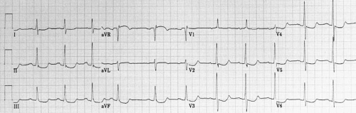 FIGURE 59.10. Left atrial abnormality. The P-wave duration is 0.125 second, and a prominent negative deflection is seen in V1. Incomplete right bundle branch block and repolarization changes induced by digitalis are also present. |
Abnormal Electrocardiogram
QRS Axis Deviation
Although QRS axes between 0 and –30 degrees are sometimes called left axis deviations, they are truly a normal variant. Severe left axis deviations (QRS axes between –30 and –90 degrees) are considered abnormal, but they are found in 2% of healthy adults (63).
Although the term left axis deviation is often used interchangeably with left anterior fascicular block (LAFB), left superior displacement of the QRS axis may occur in the absence of LAFB (in inferior myocardial infarction and other disorders). The extent of left axis deviation may vary over short periods of time, perhaps from conduction delays affecting selectively different groups of fibers in the fan-like anterior division of the left bundle branch.
P-Wave Abnormalities
Abnormalities of the P wave reflect disorders of atrial pressure or volume, or an anomalous origin of the cardiac impulse.
Right Atrial Abnormality
Right atrial enlargement has classically been diagnosed in the presence of the following: (a) tall, peaked P waves in leads II, III, and aVF (≥0.25 mV in lead II) (“P pulmonale”); (b) a P-wave axis ≥75 degrees; and (c) a positive deflection of the P wave in V1 or V2 ≥0.15 mV (64). These ECG signs, however, correlate poorly with anatomic findings. The P-wave amplitude may paradoxically decrease as right ventricular hypertrophy progresses. Also, P-wave signs have relatively low sensitivity to detect “pure” right atrial enlargement. The most sensitive ECG manifestations of right atrial abnormality in patients with low prevalence of coronary disease, no chronic pulmonary disease, and no left-sided heart disease seem to be QRS changes in lead V1 (R/S ≥1; presence of Q) (in the absence of RBBB). In addition, ST-segment depression ≥0.05 mV in II or aVF (probably representing a prominent atrial repolarization (Ta) wave) is highly specific.
Left Atrial Abnormality
Left atrial enlargement is characterized by the following: (a) a notched P wave with a duration ≥0.12 second (“P mitrale”), best observed in leads II and V1; and (b) a wide terminal negative deflection in lead V1 (0.1 mV amplitude per 0.4 second duration) (Fig. 59.10). The terminal force of the P wave correlates better with left atrial volume and weight than with atrial pressure (65). No characteristic of the P wave correlates with atrial size (66). The left atrial enlargement pattern signals an intraatrial conduction disturbance; thus, the term left atrial abnormality is preferred.
The term pseudo-P pulmonale denotes a prominent P wave in inferior leads that is caused by left, rather than right, atrial abnormality. The P wave revealed is enlarged only in its terminal portion, which in V1 is markedly negative.
Biatrial Enlargement
Biatrial enlargement is characterized by tall P waves in lead II and notched and broad P waves in leads I and II, with a terminal negative deflection in V1.
Ta Wave
Ta waves may be prominent in atrial hypertrophy or infarction and during pericarditis that has not been promptly detected. In the presence of atrial enlargement, the Ta wave is prolonged and may displace the ST segment, which appears depressed.
PR Interval
A short PR interval in the presence of a normal P-wave axis suggests an abnormally rapid conduction pathway within the AV node or its surroundings (i.e., a bundle of cardiac muscle connecting atria directly with ventricles). An impulse that bypasses the AV node leads to early activation of the ventricular myocardium (ventricular preexcitation). This creates the potential for the electrical impulse to reenter into the atria, producing a tachyarrhythmia (the Wolff-Parkinson-White [WPW] syndrome). When a short PR interval is accompanied by an abnormal P-wave direction, the site of impulse origin has moved from the sinus node to a position closer to the AV node. A prolonged PR interval with a normal P-wave axis indicates a delay in impulse transmission at some point in the pathway between the atrial and ventricular myocardium.
QRS Complex
The absence of R-wave progression from V1 to V5 may indicate LV necrosis. In precordial leads, the notching or slurring of the QRS complex is more sensitive than the presence of Q waves to detect anterior infarction, but it is less specific (67). A cause of apparent loss of left precordial R waves is the rightward mediastinal shift induced by a left pneumothorax (68). In dextrocardia, normal R-wave progression may be observed by recording leads V1 to V5R.
Q Waves
Conditions associated with abnormal Q waves include myocardial infarction or injury, LV hypertrophy (LVH) or dilatation, and intraventricular conduction disturbances (left BBB [LBBB], ventricular pacing and WPW syndrome). Less frequent causes of Q waves include infiltrative myocardial disease, chronic obstructive pulmonary disease (in precordial leads), acute pulmonary embolism, pneumothorax, and misplacement of precordial electrodes (69).
ST Segment
Alterations of the ST segment include elevation and depression, which depend on either of the following two cellular mechanisms, or both: (a) an injury current resulting from a difference in resting membrane potentials between injured and uninjured myocardium; and (b) a voltage gradient generated by a difference in AP plateau amplitudes.
The most important cause of ST-segment elevation is myocardial injury. Another cause is ventricular asynergy, which can produce a pseudoinfarction pattern (see later) (70). Depression of the ST segment occurs during myocardial ischemia and when ventricular repolarization is altered.
QT Interval
Long QT Interval
The malfunction of cardiac channels may lead to an intracellular excess of positive ions (sodium or potassium). This excess prolongs ventricular repolarization and, consequently, the QT interval. A prolonged QTc is a predictor of cardiovascular mortality even in the absence of overt heart disease (71). Causes of long QT interval include myocardial ischemia, cardiomyopathies, hypokalemia, hypocalcemia, autonomic influences, drug effects, hypothermia, and genetics (congenital long QT syndrome).
Ischemia
Acute myocardial ischemia may induce an initial, transient QT shortening followed by extreme QT prolongation. Changes in the QT interval often accompany T-wave or U-wave inversion (72). The QT interval usually normalizes within 72 hours, while inverted T waves may persist.
Hypertrophic Cardiomyopathy
The QT and QTc are prolonged in patients with hypertrophic cardiomyopathy, as a consequence of the increased LV mass (73).
Hypothermia
Hypothermia (core temperatures ≤35°C) is associated with sinus bradycardia, which, in turn, is associated with prolongation of the QT interval. In some patients, however, the QTc interval is also abnormal.
Autonomic Dysfunction
Patients with diabetes, alcoholism, and other disorders that cause autonomic dysfunction may show prolonged QT and QTc intervals (74).
Drugs
Antiarrhythmic drugs, the antibiotics erythromycin and ketoconazole, the antihistamine agents astemizole and terfenadine, the phenothiazines, and terodiline all have been associated with prolongation of both the QT and QTc intervals, with torsade de pointes, and with sudden death (75). When new drugs are under clinical development, it is important to test for a propensity to dangerous arrhythmias such as torsade. Because this is unfeasible, regulatory agencies instead require testing for drug-related changes in the QT interval (76). Recently, the selective serotonin reuptake inhibitors and the newer antipsychotic agents (e.g. clozapine, risperidone) have been reported to be associated with arrhythmias and prolonged QTc interval (77). A list of drugs associated with QT-interval prolongation is continuously updated on the Internet (78).
Congenital Long QT Syndrome
Various mutations in ion channel genes cause congenital long QT syndrome (QTc > 0.46 seconds). Five to 10% of gene carriers for this disorder, however, have QTc durations within normal range (79). Patients with the syndrome may also have marked sinus bradycardia. The T wave is often notched or biphasic, or it alternates its morphology or polarity (T-wave alternans) (80,81,82). Prominent U waves may also be present. The extreme prolongation of the QT interval can result in pseudo 2:1 AV block when every other P wave falls during or before the preceding T wave (29). The long QT-3 variety seems to be caused by mutations in the SCN5A gene, which may also underlie the Brugada syndrome.
Short QT interval
In the short QT syndrome, QTc intervals measure less than 320 milliseconds (83). Patients (including children) have a high incidence of ventricular tachyarrhythmias, syncope, sudden cardiac death, or atrial fibrillation. The condition may be associated with missense mutations in KCNH2 (HERG).
T Wave
Abnormalities of the T wave (usually consisting of inverted T waves) are seen in a number of conditions. The T wave is a sensitive detector of repolarization differences over the myocardium, but the magnitude of T-wave changes is not proportional to the extent of myocardium with repolarization abnormalities (9,84). Negative T waves have classically been classified in primary when they result from changes in the duration, shape, or amplitude of ventricular action potentials (as in ischemia, myocarditis, pericarditis, drug effects), and as secondary when changes affect not the ventricular action potential but the activation sequence (as in BBB, ventricular pacing, ventricular hypertrophy, cardiomyopathies, and WPW syndrome) (9,85). This mechanistic dichotomy, however, may be challenged in light of the phenomenon of T-wave memory and perhaps also by that of T-wave alternans, changes that could result from a combination of mechanisms or from “ventricular electrical remodeling” (86).
The term T-wave abnormality has been called into question by the finding that negative T waves that develop in infarct-related ECG leads shortly after thrombolysis are associated with improved survival (87). It appears, however, that such T waves must be dynamic (i.e., revert to positive over time, with exercise, or with dobutamine) to predict myocardial viability and favorable outcome (88,89). Abnormalities of the T wave
on a resting ECG of male patients have been shown, conversely, to predict cardiovascular mortality (90).
on a resting ECG of male patients have been shown, conversely, to predict cardiovascular mortality (90).
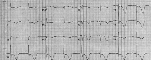 FIGURE 59.11. Memory T waves in a patient with complete atrioventricular block in whom a permanent pacemaker had been temporarily inhibited. The intrinsic rhythm shows a right bundle branch block pattern with deep, wide, negative T waves (positive in aVR) that follow the QRS morphology of the previously paced QRS complex. |
Less than 1% of ECGs recorded for any reason show giant, rather permanent negative T waves. They usually correlate with LVH or coronary disease (91).
Stay updated, free articles. Join our Telegram channel

Full access? Get Clinical Tree


