Echocardiography: Introduction
The term echocardiography refers to the evaluation of cardiac structure and function with images and recordings produced by ultrasound. In the past 30 years, it has become a fundamental component of the cardiac evaluation. Currently, echocardiography (echo) provides essential (and sometimes unexpected) clinical information and is the second most frequently performed diagnostic procedure.1 A one-dimensional (1D) method performed from the precordial area to assess cardiac anatomy has evolved into a two-dimensional (2D) modality performed from either the thorax (TTE) or from within the esophagus (TEE), capable of also delineating flow and deriving hemodynamic data.2 Newly evolving technical developments have extended the capacity of ultrasound to routine three-dimensional (3D) visualization3 and the assessment, in conjunction with contrast agents,4 of myocardial perfusion.
The development of echocardiography is usually credited to Elder and Hertz in 1954.5 For nearly two additional decades, clinical echocardiography consisted primarily of 1D time-motion (M-mode) recordings, as popularized by Feigenbaum.6 In the mid-1970s, Bom and colleagues7 developed a multielement linear-array scanner that could produce anatomically correct images of the beating heart. 2D images of superior quality were soon achieved by mechanical sector scanners8 and ultimately by phased-array instruments developed by VonRamm and Thurstone9 as the present-day standard. Recently, 3D instruments capable of real-time volumetric imaging have been developed.10 Miniaturization of ultrasound transducers has also led to handheld echographs that can be carried in a lab coat and incorporation into gastroscopes and cardiac catheters to achieve transesophageal and intravascular images.11,12
Although efforts to use the Doppler principle to measure flow velocity by ultrasound were begun in the early 1970s by Baker,13 clinical application of this technique did not thrive until the work of Hatle in the early 1980s.14 Pulsed and continuous-wave Doppler recordings soon were expanded to full 2D color-flow imaging. Most recently, Doppler velocity recordings have been obtained from myocardium itself, enabling measurement of tissue velocities and the derivation of values for regional strain.
Principles of Echocardiography
Sound is an energy form that travels through a medium as a series of alternating compressions and rarefactions of the molecules (Fig. 18–1). It is typically characterized by its wavelength, which is the distance between any two consecutive phases of the cycle (eg, peak compression to peak compression), and by its frequency, which is the number of wavelengths per unit time (customarily expressed as cycles per second, or hertz [Hz]). The velocity of sound is the product of wavelength and frequency; thus there is an inverse relationship between these two characteristics: the greater the frequency, the shorter the wavelength. Ultrasound is sonic energy with a frequency more than the audible range of the human ear (>20,000 Hz) and is useful for diagnostic imaging, because, like light, it can be directed as a beam that obeys the laws of reflection and refraction.15,16 Thus an ultrasound beam travels in a straight line through a homogeneous medium. If the beam meets an interface of different acoustic impedance, however, part of the energy reflects, and the remaining attenuated signal is transmitted. The reflected energy, or echo, is used to construct an image (Fig. 18–2).
Figure 18–1
Sound energy results in alternating compression and rarefaction of particles in a conducting medium. This alternation, which can be plotted against time (or distance), conforms to a sine-wave pattern (bottom panel). Reproduced with permission from Hagan AD, DeMaria AN. Clinical Applications of Two-Dimensional Echocardiography and Cardiac Doppler. Boston, MA: Little, Brown; 1989.
Figure 18–2
Upper panel: Attenuation of an ultrasound beam emitted from a transducer. There is reflection and progressive loss of energy at each interface encountered. Lower panel: The reflected wavefronts are recorded as signals of varying amplitudes (A mode) via the piezoelectric crystal. Upper panel modified with permission from Hagan AD, DeMaria AN. Clinical Applications of Two-Dimensional Echocardiography and Cardiac Doppler. Boston, MA: Little, Brown; 1989.
The transducer is responsible for both transmitting and receiving the ultrasound signal. The transducer consists of electrodes and a piezoelectric crystal, whose ionic structure results in deformation of shape when exposed to an electric current. Thus piezoelectric crystals are composed of synthetic materials, such as barium titanate, which, when exposed to electric current from the electrodes, alternately expand and contract to create sound waves. When subjected to the mechanical energy of sound returning from a reflecting surface, the same piezoelectric element changes shape, thereby generating an electrical signal detected by the electrodes (Fig. 18–3). Thus the transducer both produces and receives ultrasonic signals.
Figure 18–3
The basic principle of ultrasonic imaging. The piezoelectric crystal is activated, producing a transmitted pulse (T), which reflects off the interface. The reflected pulse (R) excites the crystal, producing an electric current. Because the velocity of the pulse is constant, distance can be calculated based on the transit time. (Because the pulse must travel back and forth from the interface, the time is divided by 2.) Modified with permission from Weyman.20
In the past, echographs have both transmitted and received signals of the same frequency. Recently, harmonic imaging, in which ultrasound energy is transmitted at a baseline (fundamental) frequency but then received at a higher multiple (harmonic) of that frequency (usually the first harmonic) has been implemented to enhance the signal-to-noise ratio. Harmonic imaging is based on the change in the ultrasound frequency of a transmitted wave induced by the interaction with a reflecting target. The sinusoidal waveform becomes peaked as it travels through tissue, thereby undergoing a change in frequency.
A simplistic analogy of this phenomenon would be the morphologic changes seen in ocean waves as they approach the shore and are affected by the rising ocean floor. The cresting of the waves (the tops move more rapidly than the bases) and the changes in their height are analogous to the harmonic signals generated by the interaction of ultrasound and tissue. These signals take some time (and distance) to develop. Therefore, structures close to the transducer do not generate much harmonic signal at all, and thus near-field artifacts and reverberation artifacts are minimized.
Harmonic imaging has also been very useful in conjunction with intravascular echo contrast agents. These microbubbles demonstrate cyclic expansion and constriction during ultrasound imaging, and this resonance produces a large amount of harmonic energy.17 In contrast, myocardial tissue does not resonate to any appreciable degree. The net effect of harmonic imaging with echocardiographic contrast is a marked enhancement of the signal from the left ventricular (LV) cavity and/or the coronary microcirculation compared with that of the myocardium.
Ultrasound presents several unique technical difficulties. Sound energy is poorly transmitted through air and bone, and the ability to record adequate images depends on a thoracic window that gives the interrogating beam adequate access to cardiac structures. The degree to which ultrasonic energy is reflected depends on how perpendicular the interrogating beam is to the interface. When the ultrasound beam is directed parallel to the interface, little or no sound energy reflects to the transducer. Therefore, poor signal transmission, a nonorthogonal orientation of the ultrasound beam to the surface, and energy attenuation can cause failure to record signals from cardiac structures—a phenomenon referred to as echo dropout.18 Conversely, some structures may be such strong ultrasonic reflectors, being extremely dense and usually perpendicular to the beam, that sufficient energy returns to the transducer to reflect and again transmit into the field. This phenomenon can lead to reverberations, or the reproduction of the echoes of anatomic structures at multiple locations within the image.19 Finally, very dense targets lying on the periphery of a 2D-sector ultrasound beam may be recorded and displayed as if they were located along the central scan line (Fig. 18–4). This problem may be accentuated in the setting of strong reflectors that result in the formation of side lobes.20
Figure 18–4
Upper panel: The transducer emits an ultrasonic beam that has a near field (where the beam is relatively focused) and a far field (where the beam width increases). Lower panel: B-mode diagram showing the effect of beam width. In the near field, the beam reflects off only 1 of 2 objects in close proximity to each other. In the far field, however, 2 similarly positioned objects are both within the beam width. Therefore, lateral resolution is compromised, and the objects’ positions are misrepresented.
The construction of a cardiac image from ultrasound signals is based on computation of the distance between an anatomic structure and the transducer (see Fig. 18–3). Thus an ultrasound beam is produced by a handheld transducer positioned on the thorax and directed into the heart. This beam travels in a straight line until it reaches an interface between structures of different acoustic impedance, such as blood and myocardium. At this point, some ultrasonic energy reflects, some scatters, and some continues forward. The amplitude of the propagating signal is attenuated because of the reduction in energy at the interface (see Fig. 18–2). Electronic circuitry within the echograph measures the time interval required for the transit of the ultrasound beam from the transducer to the interface and back again. Because the velocity of sound in soft tissue is constant (~1540 m/s), the instrument can calculate the total distance traveled to and from the reflecting surface as the product of transit time and velocity of sound. Interface location is derived as one-half of the total transit distance, and a signal is depicted on an oscilloscope or video monitor at that point (see Fig. 18–3). The amplitude of ultrasonic energy reflected from each target interface is represented by the brightness of the signal that is displayed.
In the most basic form of echocardiography, a single scan line produced by a piezoelectric crystal is passed through the heart (Fig. 18–5). At each structural interface, ultrasonic energy is reflected back and displayed at the appropriate distance as a signal, the amplitude of which represents the acoustic impedance or density of the material encountered. These signals are subsequently displayed as dots, the brightness of which is proportional to the amplitude of reflected ultrasonic energy. Accordingly, if repetitive B-mode scan lines are produced and swept across the screen over time, the movement of the heart can be obtained as a time-motion (or M-mode) recording, providing dynamic cardiac images (see Fig. 18–5). In clinical use, the piezoelectric crystal within the transducer is activated by alternating electric current to transmit at a rate of approximately 1000 pulses/s. This same crystal also receives the returning echo reflections and actually spends most of the time (>90%) in the receive rather than the transmit mode. Because it transmits ultrasound signals at 1000 pulses/s, M-mode echocardiography provides very high temporal resolution and is excellent for timing cardiac events or recording high-velocity motion. 2D echocardiography acquires multiple B-mode scan lines that are aligned in the appropriate anatomic location to form a wedge-shaped sector image that provides additional spatial information in either superoinferior or mediolateral directions.
Figure 18–5
Formation of A-mode, B-mode, and M-mode echocardiograms. The transducer emits an ultrasound beam, which reflects at each anatomic interface. The reflected wavefronts can be represented as dots (B mode) or spikes (A mode). The dot brightness and spike magnitude vary with the amplitude of the reflected wave. If the B-mode scan is swept from left to right with time, an M-mode image is produced. AML, anterior mitral leaflet; CW, chest wall; IVS, interventricular septum; PML, posterior mitral leaflet; PW, posterior wall; RV, right ventricle. Modified with permission from Hagan AD, DeMaria AN. Clinical Applications of Two-Dimensional Echocardiography and Cardiac Doppler. Boston, MA: Little, Brown; 1989.
High-quality images require optimal resolution—that is, the ability to distinguish two individual objects separated in space. Short wavelengths yield excellent resolution in echo imaging, because the shorter the cycle length, the smaller the object that will reflect the signal and be detected by the echo scanner. Because wavelength is inversely related to frequency, transducers that emit a high-frequency signal (≥3.5-7.0 MHz) yield high-resolution images. Because ultrasonic beams diverge as they propagate away from the transducer, the width of the beam can become sufficiently great to encompass multiple targets and decrease resolution (see Fig. 18–4). The degree of beam divergence is also less with high-frequency sonic energy than with low-frequency signals. The smaller wavelengths associated with high-frequency signals, however, are subject to greater reflection and scattering, with substantially higher attenuation as the beam propagates through tissue. The resultant attenuation is greater and leads to decreased sensitivity. Therefore, in clinical practice, echocardiographic examinations are performed using the highest-frequency transducer capable of sufficient penetration to obtain signals from all potential targets within the ultrasound field.
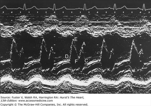
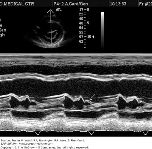
Despite the availability of 2D imaging, M-mode echocardiography remains a useful part of the ultrasound examination. Figure 18–6 show the typical views obtained when the transducer is placed at the left parasternal area and rocked through the heart from apex to base. Tissue typically reflects ultrasound at its surface (specular reflectors) and from internal inhomogenicity (backscatter), whereas blood is homogenous and does not produce reflections. At the mitral valve (MV) level (Fig. 18–6C), the cardiac structure seen closest to the transducer is the right ventricular (RV) free wall; it is followed by the RV cavity, the interventricular septum, the MV apparatus, and the LV posterior wall as the beam travels backward. At this level, MV excursion is well seen and is more easily recorded for the longer anterior leaflet. For the anterior leaflet, diastolic mitral opening is bipeaked (M-shaped), with maximal opening during early diastolic filling at the E point, a subsequent reclosure downslope to the F point, and a reopening with atrial contraction at the A point before valve closure at the C point21 (Fig. 18–7). The posterior leaflet manifests a mirror-image W-shaped pattern. When LV end-diastolic pressure is elevated, a shoulder (B bump) is often present between the A and C points (Fig. 18–8). If the transducer beam is directed inferolaterally from the MV level, the papillary muscles and LV apex are imaged (see Fig. 18–6A). With superior and medial angulation, the left atrium (LA), aortic valve (AoV), and aortic root (AO) are seen. The tricuspid valve (TV) can be imaged by angulating the transducer inferomedially and the pulmonic valve (PV) by angulating slightly superiorly and laterally.
Figure 18–6

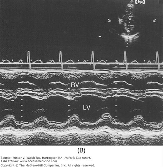
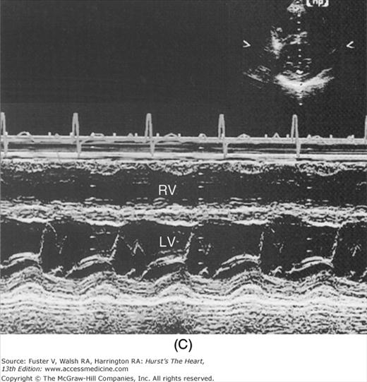

A. Diagram of an M-mode sweep from apex to base in a normal heart (parasternal view). B. to D. M-mode sweep from apex to base in a normal individual. aMVL, anterior mitral valve leaflet; Ao, aorta; AoV, aortic valve; APS, atriopulmonic sulcus; ARVW, anterior right ventricular wall; ATVL, anterior tricuspid valve leaflet; AVJ, atrioventricular junction; Ch, chordae tendineae; EN, endocardium; E,P, epicardial/pericardial interface; IVS, interventricular septum; LA, left atrium; LAW, left atrial wall; LV, left ventricle; LVOT, left ventricular outflow tract; PA, pulmonary artery; PMVL, posterior mitral valve leaflet; PPM, posterior papillary muscle; PV, pulmonic valve; RA, right atrium; RV, right ventricle; RVOT, right ventricular outflow tract. A, reproduced with permission from Felner JM, Schlant RC. Echocardiography: A Teaching Atlas. New York, NY: Grune & Stratton; 1976.
Measurements of the LV cavity dimension and wall thickness can be readily derived from M-mode recordings (Fig. 18–9) and are usually made according to the recommendations of the American Society of Echocardiography (ASE) at end diastole (the onset of the QRS complex) and end systole (the point of maximum upward motion of the LV posterior wall endocardium).22 Measurements should be made from leading edge to leading edge. They are accurate if the beam is orthogonal to the long axis of the ventricle. By convention, left atrial dimension is measured at end systole, and AO diameter is recorded at end diastole at the level of the base of the heart (see Fig. 18–9). During systole, opening of the aortic leaflets appears as a parallelogram produced by motion of the right coronary and (usually) the noncoronary AoV cusps.
Figure 18–9
Recommended criteria for M-mode measurement of cardiac dimensions (see text for details). The figure and the elliptical inserts (a, b, c, d, and e) illustrate the leading-edge method. aMVL, anterior mitral valve leaflet; Ao, aorta; AoV, aortic valve; ARV, anterior right ventricular wall; EN, endocardium; EP, epicardium; LA, left atrium; LV, left ventricle; PLV, posterior left ventricular (wall); PPM, papillary muscle; PMVL, posterior mitral valve leaflet; RV, right ventricle; S, septum. Reproduced with permission from Sahn et al.22
The M-mode LV cavity dimensions can be used to estimate ventricular volumes and ejection fraction (EF) if desired, most simply by merely cubing the value (D3). Such calculations involve several assumptions regarding LV geometry that are not uniformly valid.23 The fractional shortening can also be determined.24 This value is often helpful in assessing systolic function, but it reflects the function of the LV in one chord and in one plane and can be misleading with asynchronous contraction.25 An additional M-mode marker of systolic function is E-point to septal separation, or the distance between the anterior MV leaflet at its most anterior opening excursion (the E point) and the interventricular septum. A value of 8 mm or greater is abnormal.26 The normal M-mode measurements are seen in Table 18–1.
| Mean ± Standard Deviation | Range | Mean ± Standard Deviation | Range | |
|---|---|---|---|---|
| No. of patients | 25 | — | 50 | — |
| Age, years | 10 ± 3 | 4-18 | 24 ± 0.6 | 1.10-2.53 |
| BSA, m2 | 1.33 ± 0.38 | 0.72-2.04 | 1.81 ± 0.34 | 1.10-2.53 |
| LVIDd, mm | 44 ± 6 | 32-50 | 50 ± 3 | 42-60 |
| LVIDs, mm | 28 ± 7 | 32-50 | 50 ± 3 | 22-43 |
| FSLV | 34 ± 4 | 25-42 | 33 ± 3 | 28-37 |
| IVS thickness, mm | 8 ± 2 | 5-10 | 9 ± 1 | 7-12 |
| IVS excursion, mm | 7 ± 1 | 5-9 | 9 ± 1 | 7-12 |
| PWd thickness, mm | 7 ± 2 | 4-9 | 9 ± 1 | 7-12 |
| PWs thickness, mm | 12 ± 3 | 8-17 | 16 ± 2 | 13-20 |
| α thickening PW | 0.70 ± 0.25 | 0.41-0.95 | 0.50 ± 0.19 | 0.32-0.69 |
| PW excursion, mm | 9 ± 2 | 7-14 | 11 ± 2 | 9-17 |
| RVDd supine, mm | — | — | 15 ± 6 | 7-22 |
| RVDd left lateral, mm | — | — | 20 ± 8 | 10-37 |
| Aortad mm | 23 ± 4 | 15-27 | 28 ± 5 | 26-36 |
| LADs mm | 25 ± 5 | 20-31 | 27 ± 6 | 12-35 |
Multiple individual B-mode scan lines can be rapidly transmitted, received, and displayed in appropriate spatial orientation to construct a 2D image of the heart. The initial approach simply used a linear array of 20 piezoelectric crystals placed side by side, each of which transmitted and received signals independently (Fig. 18–10A). The resulting scan lines were displayed simultaneously to yield rectangular images.
Figure 18–10
The four major types of ultrasonic scanners used to acquire 2D echocardiographic images. A. Linear-array scanner. B. Oscillating scanner. C. Rotating mechanical scanner. D. Phased-array scanner. Reproduced with permission from Hagan AD, DeMaria AN. Clinical Applications of Two-Dimensional Echocardiography and Cardiac Doppler. Boston, MA: Little, Brown; 1989.
Current 2D scanners use B-mode scan lines that are independently transmitted and received and are directed through a wedge-shaped sector of cardiac anatomy by means of mechanical or electrical beam steering (see Fig. 18–10A,B). A variety of motorized devices can mechanically direct multiple scan lines through a sector arc of the cardiovascular system, positioning the beam in space by determining the orientation of the piezoelectric crystal. Most current 2D scanners use a phased-array approach, where multiple ultrasonic crystals are used in concert to create individual B-mode scan lines. The crystals are activated in a closely coordinated temporal sequence, so that the individual wavelets produced by each element merge to form a single beam, the direction of which is determined by the sequence of crystal firing (Fig. 18–11). The beam can be electrically swept throughout a 90-degree sector arc. Also, a firing sequence can be used that results in dynamic focusing of the beam along its length to achieve minimal beam width and increased resolution. Phased-array 2D scanners use small transducers with no moving parts that could require repair.
Figure 18–11
Electronic steering of a phased-array ultrasound beam. A. Elements are fired in sequence from left to right, resulting in a beam directed to the left. B. Elements are fired in sequence opposite to those in (A), producing a beam directed to the right. C. Elements are fired from the periphery toward the center, producing a beam that converges on a given focal point. Reproduced with permission from Hagan AD, DeMaria AN. Clinical Applications of Two-Dimensional Echocardiography and Cardiac Doppler. Boston, MA: Little Brown; 1989.
Originally, echocardiographic data were displayed in analog form on a standard oscilloscope, transferred to a video monitor by a television camera, and hard-copied onto videotape or paper. Currently, computerized analog-to-digital scan conversion is standard, so the polar signals of individual scan lines are converted to a series of numerical gray-level values for individual box-like picture elements (pixels) aligned along X-Y coordinates.27 The ability of a digital step-gradation technique to reproduce the continuous gradation of analog methods is a function of the density of pixels in the matrix and the gray-level shades available. The digital format provides the opportunity for image processing, enhancement, and quantitation. Storage in digital format can avoid the image degradation inherent in videotape, provide random access and easy comparison of studies, enable rapid image transmission, and prevent deterioration with image copying and prolonged storage. Fully digital acquisition and storage of echocardiograms is now commonplace and much more convenient than analog videotape recordings.
To help standardize the 2D examination, the ASE recommends that cardiac imaging be performed in three orthogonal planes:
Long-axis (from AO to the apex)
Short-axis (perpendicular to long axis)
Four-chamber (traversing both ventricles and atria through the mitral and tricuspid valves)28 (Fig. 18–12)
Figure 18–12
The three basic tomographic imaging planes used in echocardiography: long axis, short axis, and four chamber. Ao, aorta; LA, left atrium; LV, left ventricle; PA, pulmonary artery; RA, right atrium; RV, right ventricle. Reproduced with permission from Hagan AD, DeMaria AN. Clinical Applications of Two-Dimensional Echocardiography and Cardiac Doppler. Boston, MA: Little, Brown; 1989.
The long and short axes are those of the heart, not the body. These three planes can be visualized using four basic transducer positions: parasternal, apical, subcostal, and suprasternal (Fig. 18–13). The four-chamber views are obtained from the apical and subcostal positions. The ASE recommends that an image obtained within 45 degrees of a basic orthogonal plane be identified with that orthogonal plane. Table 18–2 lists the standard transducer positions and transthoracic echocardiographic (TTE) views. Anatomic drawings of the various imaging planes are seen in Figs. 18–13, 18–14, 18–15, 18–16, 18–17, 18–18, 18–19, 18–20.
| Parasternal position |
| Long axis |
| Left ventricular long axis |
| Right ventricular long axis |
| Right ventricular outflow |
| Short axis |
| Short axis through the plane of the |
| Cardiac base |
| Mitral valve |
| Chordae tendineae |
| Papillary muscles |
| Apex |
| Apical position |
| Four-chamber plane |
| Five-chamber plane |
| (Four-chamber plane angled superiorly to include the aorta) |
| Two-chamber plane |
| Three-chamber plane |
| Subcostal position |
| Four-chamber plane |
| Short axis through the plane of the |
| Mitral valve |
| Papillary muscles |
| Cardiac base |
| Posteriorly directed planes through the venae cavae and atria |
| Suprasternal position |
| Long axis (through the ascending and descending aorta) |
| Short axis |
Figure 18–13
Visualization of the heart’s basic tomographic imaging planes by various transducer positions. The long-axis plane (A) can be imaged in the parasternal, suprasternal, and apical positions; the short-axis plane (B) in the parasternal and subcostal positions; and the four-chamber plane (C) in the apical and subcostal positions. Reproduced with permission from Henry et al.28
The echocardiographic examination is iterative and largely determined by the anatomic characteristics of the patient and manual manipulation of the transducer by the operator. Of paramount importance is the identification of a thoracic site (window) that enables transmission of the ultrasound signal to the heart. The echocardiographic examination may be performed with the operator either to the patient’s left or right. The patient is in the left lateral decubitus position for most of the examination, with the head of the bed elevated 20 to 30 degrees.
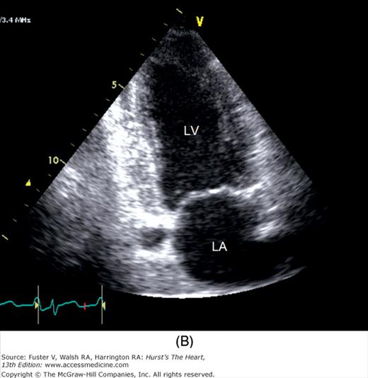
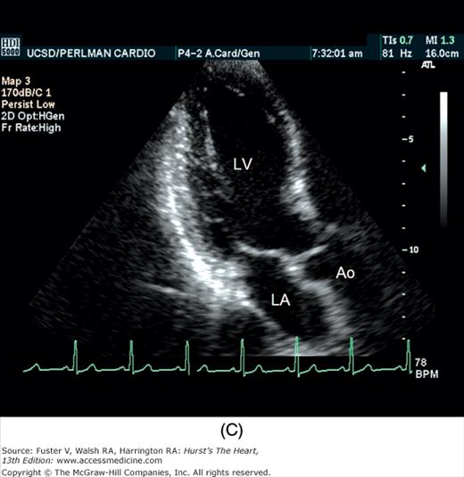
The examination customarily begins with the transducer in the left parasternal position in the long-axis view (Fig. 18–14). This provides excellent images of the LV, aorta, LA, and the mitral and aortic valves. By angling the beam slightly rightward and inferiorly (RV inflow view), the right atrium (RA), RV, and TV are visualized (Fig. 18–15).
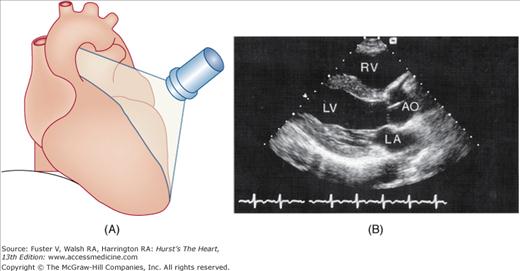
Figure 18–15
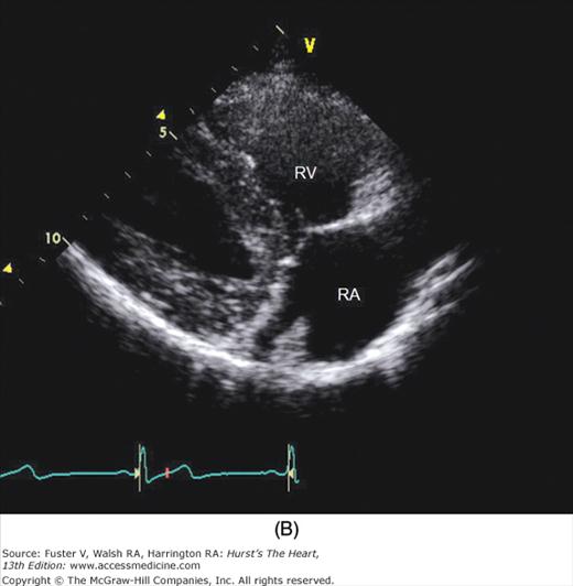
A. Orientation of the sector beam and transducer position for the parasternal RV inflow plane. B. Two-dimensional image of RV inflow plane. RA, right atrium; RV, right ventricle. A, reproduced with permission from Hagan AD, DeMaria AN. Clinical Applications of Two-Dimensional Echocardiography and Cardiac Doppler. Boston, MA: Little, Brown; 1989.
A 90-degree clockwise turn of the transducer produces the parasternal short-axis view. Slight axial angulation of the transducer enables visualization of the LV at various levels of the short axis, including the papillary muscle, mitral leaflets, and AoV (Fig. 18–16). With angulation toward the base, the LA, right heart structures, main pulmonary artery (PA), and occasionally the LA appendage are also recorded. The apical views are best acquired with the patient in a steep left lateral decubitus position and the transducer at the point of the apical impulse. The four-chamber view is obtained by turning the transducer so that both ventricles, atrioventricular valves, and atria are visualized (Fig. 18–17). In this view, the septal, apical, and lateral walls of the LV are visualized. Slight superior angulation of the transducer will add the AoV and proximal ascending aorta to the echocardiographic image (apical five-chamber view). From the four-chamber view, 90 degrees of counterclockwise transducer rotation produce the apical two-chamber view (Fig. 18–18A,B). This imaging plane demonstrates the LA and the inferior, apical, and anterior wall segments of the LV (the right heart structures are absent). If the transducer is rotated slightly further, a three-chamber view similar to the parasternal long-axis view is produced (Fig. 18–18C) and provides images of the posterior, apical, and anteroseptal LV wall segments, as well as the LA, aorta, and mitral and aortic valves.
Figure 18–16
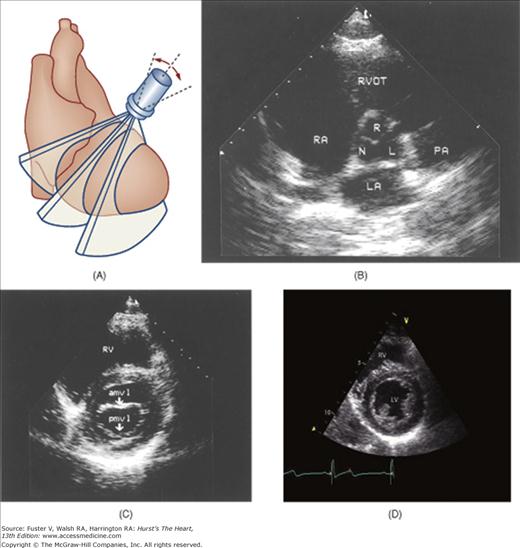
A. Orientation of various short-axis sector beams through the left ventricle obtained by angling the transducer in the parasternal position. B. Short-axis plane through the base of the heart. C. At the level of the mitral valve leaflets. D. At the papillary muscle level. E. Modified parasternal short axis plane through the RV outflow tract and pulmonary artery. aMVL, anterior mitral valve leaflet; L, left cusp of the aortic valve; LA, left atrium; LV, left ventricle; N, noncoronary cusp of the aortic valve, PA, pulmonary artery; PMVL, posterior mitral valve leaflet; RA, right atrium; R, right cusp of the aortic valve; RV, right ventricle; RVOT, right ventricular outflow tract. A, reproduced with permission from Hagan AD, DeMaria AN. Clinical Applications of Two-Dimensional Echocardiography and Cardiac Doppler. Boston, MA: Little, Brown; 1989.
Figure 18–17
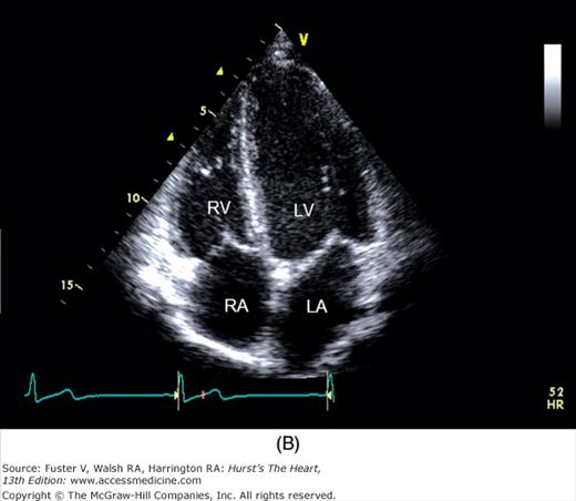
A. Orientation of the sector beam and transducer position for the apical four-chamber plane. B. 2D image of the apical four-chamber plane. LA, left atrium; LV, left ventricle; RA, right atrium; RV, right ventricle. A, reproduced with permission from Hagan AD, DeMaria AN. Clinical Applications of Two-Dimensional Echocardiography and Cardiac Doppler. Boston, MA: Little, Brown; 1989.
Figure 18–18
A. Orientation of the sector beam and transducer position for the apical two-chamber plane. B. 2D image of the apical two-chamber plane. C. 2D image of the apical three-chamber view. Ao, aorta; LA, atrium; LV, left ventricle. A, reproduced with permission from Hagan AD, DeMaria AN. Clinical Applications of Two-Dimensional Echocardiography and Cardiac Doppler. Boston, MA: Little, Brown; 1989.
To facilitate subcostal imaging, the patient is moved into a supine position. The subcostal four-chamber view is much like the apical four-chamber view (Fig. 18–19), but because the ultrasound beam is now more perpendicular to the interventricular and interatrial septa, subcostal imaging is often helpful in the examination of these structures. A 90-degree rotation of the transducer will record a subcostal short-axis view. The transducer can also be angled to image the RV outflow and PA as well as the inferior vena cava (see Fig. 18–19).
Figure 18–19
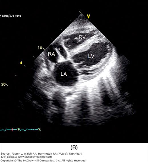
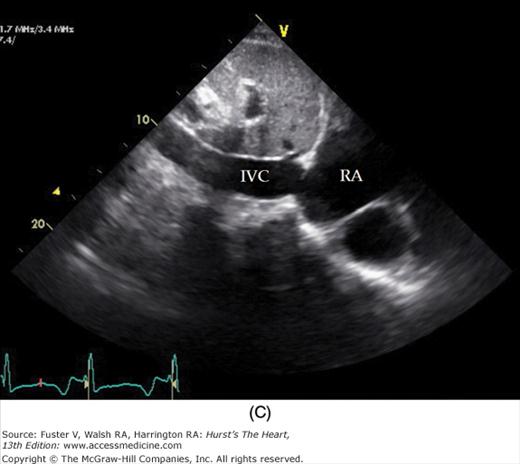
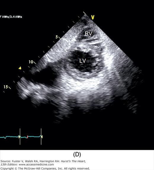
A. Orientation of the sector beam and transducer position for the subcostal four-chamber plane. B. 2D image of the subcostal four-chamber plane. C. Subcostal 2D image demonstrating the right atrium (RA) and inferior vena cava (IVC). D. 2D image of the subcostal short-axis plane. Asterisk, a prominent eustachian valve; LA, left atrium; LV, left ventricle; RA, right atrium; RV, right ventricle. A, reproduced with permission from Hagen AD, DeMaria AN. Clinical Applications of Two-Dimensional Echocardiography and Cardiac Doppler. Boston, MA: Little, Brown; 1989.
The long-axis suprasternal imaging plane is shown in Fig. 18–20. In adults the LV is usually not visualized satisfactorily from the suprasternal position, but these imaging planes are well suited for examination of the thoracic aorta, PA, and great vessels. Normal values for 2D echocardiographic measurements are shown in Table 18–3.
| Cardiac Feature | Range | Mean | Index (cm/m2) |
|---|---|---|---|
| Apical four-chamber view | |||
| LVd major | 6.9-10.3 cm | 8.6 cm | 4.1-5.7 |
| LVd minor | 3.3-6.1 cm | 4.7 cm | 2.2-3.1 |
| LVs minor | 1.9-3.7 cm | 2.8 cm | 1.3-2.0 |
| LVd area | 21.2-40.2 cm2 | 31.2 cm2 | — |
| LVs area | 8.0-21.1 cm2 | 14.2 cm2 | — |
| RV major | 6.5-9.5 cm2 | 8.0 cm | 3.8-5.3 |
| RV minor | 2.2-4.4 cm2 | 3.3-3.5 cm | 1.0-2.8 |
| RVd area | 12.0-22.2 cm2 | 18.6-2.1 cm2 | — |
| RVs area | 5.4-14.6 cm2 | 9.9 cm2 | — |
| LA major | 4.1-6.1 cm | 5.1 cm | 2.3-3.5 |
| LA minor | 2.8-4.3 cm | 3.5 cm | 1.6-2.4 |
| LA area | 10.2-17.8 cm2 | 14.7 cm2 | — |
| RA major (inf-sup) | 3.5-5.5 cm | 4.3-4.5 cm | 2.0-3.1 |
| RA minor | 2.5-4.9 cm | 3.7 cm | 1.7-2.5 |
| RA area | 11.3-16.7 cm2 | 13.8-14 cm2 | — |
| Apical two-chamber view | |||
| LVd major | 6.8-9.4 cm | 8.0 cm | — |
| LVd minor | 3.8-5.7 cm | 4.6 cm | — |
| LVd area | 19.4-48.0 cm2 | 35.6 cm2 | — |
| LVs | 8.9-27.0 cm | 14.3 cm | — |
| Parasternal long-axis view | |||
| LVd | 3.5-6.0 cm | 4.8 cm | 2.3-3.1 |
| LVs | 2.1-4.0 cm | 3.1 cm | 1.4-2.1 |
| RV | 1.9-3.8 cm | 2.8 cm | 1.2-2.0 |
| LA (A-P) | 2.7-4.5 cm | 3.6 cm | 1.6-2.4 |
| LA (S-I) | 3.1-5.5 cm | 4.4 cm | — |
| LA area | 9.0-19.3 cm2 | 13.8 cm2 | — |
| Ao | 2.2-3.6 cm | 2.9 cm | 1.4-2.0 |
| Parasternal short-axis view | |||
| Ao | 2.3-3.7 cm | 3.0-2.3 cm | 1.6-2.4 |
| RVOT | 1.9-2.2 cm | 2.7 cm | — |
| RA | 1.5-2.5 cm | 1.9-2.2 cm | — |
| LA | 2.6-4.5 cm | 3.6 cm | 1.6-2.4 |
| LA area | 7.2-13.0 cm2 | 10.8 cm2 | — |
| LVd (PM level) | 3.5-5.8 cm | 4.7 cm | 2.2-3.1 |
| LVs (PM level) | 2.2-4.0 cm | 3.1 cm | 1.4-2.2 |
| LVd area (PM level) | 16.0-31.2 cm2 | 22.2 cm2 | — |
| LVs area (PM level) | 5.2-13.4 cm2 | 8.5 cm2 | — |
| LVd (Ch. level) | 3.5-6.2 | 4.8 cm | 2.3-3.2 |
| LVs (Ch. level) | 2.3-4.0 | 3.2 cm | 1.5-2.2 |
| LVd area (Ch. level) | 16.4-32.3 cm2 | 22.5 cm2 | — |
| LVs area (Ch. level) | 6.1-16.8 cm2 | 10.7 cm2 | — |
| Subcostal view | |||
| IVC diameter | 1.8 cm | — | |
Several approaches exist to obtaining 3D echocardiographic images. The simplest approach is to merely move the transducer through a defined space and reconstruct an image by aligning the tomographic slices appropriately. A variety of spatial locator devices can be attached to the transducer to provide spatial orientation. Images obtained in this way can be high quality and accurate, but they require computer reconstruction and therefore cannot be displayed in real time. Nevertheless, these reconstructed 3D images can be valuable in quantifying cardiac volumes and EF, assessing congenital heart disease (CHD), and evaluating structures of complex geometry such as the RV.29 Using a transducer with a matrix array of crystals, a pyramid-shaped ultrasound beam can be produced that can often encompass the entire heart from one transducer location and acquire an entire data set in a single cardiac cycle. Although the initial images often lacked resolution, this type of real-time 3D imaging has evolved considerably, and new software advances have improved surface rendering and endocardial border definition (see Fig. 18–20C). Recent studies have shown an excellent correlation between real-time 3D echo and MRI in the measurement of regional and global LV volume and time-wall motion curves.30 Real-time 3D echo imaging may be useful for assessing regional EF and dyssynchrony (discussed in Ventricular Dyssynchrony and Cardiac Resynchronization Therapy on page 484.31 Finally, real-time 3D TEE has been implemented and can provide valuable information regarding the evaluation and repair of cardiac valves and the positioning of intracardiac prostheses (see Fig. 18–20D,F).32,33
Figure 18–20
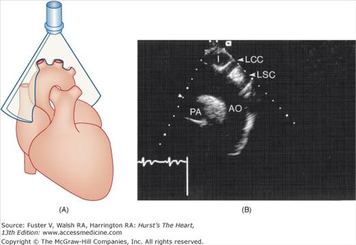
A. Orientation of the sector beam and transducer position for long-axis plane through the aorta from the suprasternal position. B. 2D image of the suprasternal long-axis view of the thoracic aorta. C. Example of 3D image in a case of dilated cardiomyopathy. D. 3D transesophageal image of the mitral valve during systole (left) and diastole (right). E. Simultaneous orthogonal TEE images of a PFO occluder device (arrow). F. 3D transesophageal image of a PFO occluder device. AL, anterior mitral valve leaflet; Ao, aorta; I, innominate artery; LCCA, left common carotid artery; LSC, left subclavian artery; LV, left ventricle; P1/P2/ P3, lateral/middle/medial scallops of the posterior mitral valve leaflet; PA, right pulmonary artery; PFO, patent foramen ovale; RA, right atrium; RV, right ventricle. D, reproduced with permission from Perk et al.31
2D echocardiography is the standard clinical approach for measuring cardiac chamber volumes and EF.34-36 Numerous algorithms have been applied to calculate LV volumes by echocardiography (Fig. 18–21). Most algorithms assumed that the LV conforms to the shape of a prolate ellipsoid or a combination of geometric shapes and calculate volume by diameter-length or area-length formulas.37 Multiple studies comparing LV volume calculated by area-length methods to those obtained by other techniques have yielded good correlations, with the best results obtained using biplane apical views.38,39 Currently, the most commonly used algorithm to calculate LV volumes is based on the Simpson rule, which derives measurements by dividing the LV by parallel planes into a number of small segments and then summating the area of the individual disks. Although all modifications of the Simpson rule give good results, the optimal correlations have been achieved with a modification that separately quantifies the volume of the apex as an ellipsoid.36,38
Accurate calculations of LV volumes by echocardiography are critically dependent on high-quality images to delineate the endocardium and image the entire LV perimeter. Echocardiographic estimates of LV volumes underestimate those calculated by other techniques and are most accurate in the absence of significant alterations of LV size and contraction. End-systolic measurements are more accurate than end diastolic, probably owing to superior endocardial definition. Nevertheless, echocardiographic calculations of LV volumes have generally yielded correlation coefficients in excess of 0.75 as compared with radionuclide angiography, cineangiography, and autopsy studies, regardless of the algorithm used.33-38 However, 2D echocardiography has been limited in the reproducibility between individual studies, especially in comparison with MRI.
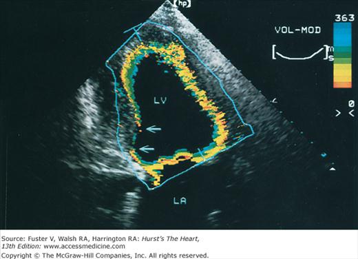
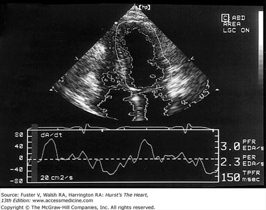
Images of the power spectrum of the Doppler signal produced by contraction/relaxation and colorization of the B-mode tissue image have been used to visualize the endocardial surface.39 Greater enhancement of endocardial border delineation and improvement of the reliability of measures of LV size and contraction have been achieved using tissue harmonic imaging and by the injection of ultrasonic contrast agents to opacify the LV cavity.40 A software package that provides instantaneous and automated endocardial border delineation throughout the cardiac cycle has been developed based on the display of tissue signals as backscatter rather than specular reflection.41 This technique of automated quantitation can yield continuous measurements of LV volume throughout the cardiac cycle and can derive values for EF, ejection rate, and rate of filling during diastole (Fig. 18–22). This same technology has been used to display endocardial excursion throughout systolic contraction or diastolic expansion in a color format superimposed on the tissue image (Fig. 18–23). This technique has been valuable in the recognition of abnormalities of LV contraction and regional disturbances of LV diastolic function.42,43 Finally, studies using 3D echocardiography have reported better reproducibility of measurements than 2D methods.
Doppler Echocardiography: Principles and Applications
Using the principle first delineated by the physicist Johann Christian Doppler,44 ultrasound can be used to determine the velocity and direction of blood flow by measuring the change in frequency produced when sound waves are reflected from red blood cells. Thus information regarding the presence, direction, velocity, and turbulence of blood flow can be acquired by cardiac ultrasound.
The Doppler principle states that when a sound (or light) signal strikes a moving object, the frequency of that signal is altered, and the increase or decrease in frequency is proportional to the velocity and direction at which the object is moving (Fig. 18–24). If a stationary transducer at the apex emits a sound wave with a transmitted frequency of fo and the wave is reflected by nonmoving red blood cells (RBCs) in an isovolumic phase of the cardiac cycle, the received frequency fr will be identical to fo. If the signal is reflected by RBCs that are moving toward the transducer, as through the MV in diastole, the returning waves will be compressed so that fr > fo. Conversely, if the target RBCs are moving away from the transducer, as in the outflow tract in systole, the returning sound waves will be elongated and the received frequency will be decreased. It is important to note that the magnitude of change in the received frequency is directly related to the velocity at which blood is flowing toward or away from the transducer.45 If the velocity of sound and the angle between the direction of RBC flow and the beam path are known, then the velocity of the RBCs is described by the Doppler equation:
Figure 18–24

Basic principle of the Doppler shift. During diastole (left panel), an ultrasound beam directed toward the junction of the mitral and aortic annuli is reflected by red blood cells moving toward the transducer. The frequency of the received ultrasound is greater than that of the transmitted beam, and the spectral tracing is recorded above the baseline (ie, flow is toward the transducer). During the isovolumic phase (middle panel), both the mitral and aortic valves are closed and little flow occurs within the left ventricle. Therefore, there are no significant changes in the transmitted and received frequencies of the Doppler beam, and no spectral tracing is recorded. During systole (right panel), the transmitted beam is reflected by red blood cells moving away from the transducer. Therefore, the frequency of the received ultrasound is lower than that of the transmitted beam, and the spectral tracing is recorded below the baseline.
V = fd (c)/2fo (cosθ)
where fd is the frequency shift recorded, fo the transmitted frequency, and c the velocity of sound. Note that the denominator is doubled. By measuring Doppler shift frequencies, the velocity and direction of blood flow can be calculated, displayed, and recorded.
The angle between the direction of blood flow and the course of the sound beam is a most important factor in Doppler ultrasound (Fig. 18–25). Velocity is a vectorial entity, having magnitude and direction, and Doppler detects only those velocities parallel or near parallel to the interrogating signal. Because the relationship between velocity and the angle is a cosine function and the cosine of angles up to 20 degrees is 0.9, little error is introduced within this range.45 However, considerable errors occur when it is >20 degrees. Moreover, the angle of incidence in 3D space usually cannot be determined with certainty from 2D echocardiographic images. Therefore, it is crucial to position and direct the transducer so that the beam is as parallel to flow as possible. In clinical use, the frequency of transmitted ultrasound is in the range of 2 to 7 MHz, the velocity of sound in tissue is approximately 1540 m/s, and the Doppler shift frequency is relatively small (~1–4 kHz) as compared with the transmitted frequency. Because the Doppler shift frequencies are in the audible range, a speaker integrated into the Doppler echocardiography system can present them as an audible signal. Normal signals are tonal or musical.
Figure 18–25
Effect of the angle of incidence on the velocity recorded with Doppler analysis. The true velocity is underestimated when the ultrasound beam is not parallel to the direction of blood flow. Reproduced with permission from Hagan AD, DeMaria AN. Clinical Applications of Two-Dimensional Echocardiography and Cardiac Doppler. Boston, MA: Little, Brown; 1989.
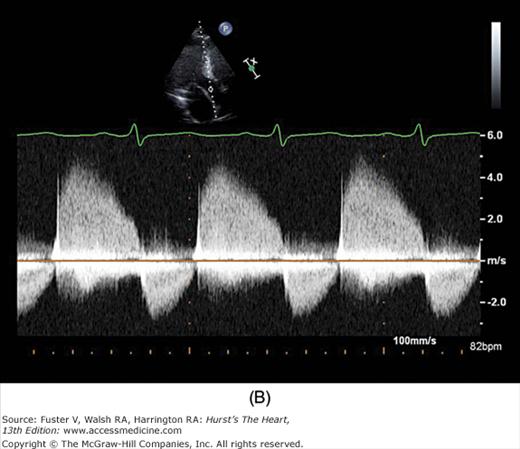
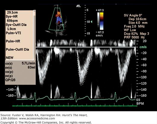
Figure 18–26 shows the typical graphic pulsed Doppler pattern of normal systolic blood flow through the RV outflow tract into the PA, with flow velocity on the y-axis and time on the x-axis. The location and size of the area from which Doppler recordings are derived is determined by positioning a sample volume on the echo image. The absence of flow is represented by the zero or no-flow line, termed the baseline. By convention, flow toward the transducer is displayed above the baseline and flow away from the transducer is displayed below the baseline. The velocities above and below baseline represent flow toward or away from the transducer, not forward or backward in the circulation. The sample volume almost invariably includes RBCs flowing at slightly different velocities. Even normal laminar blood flow in the great vessels varies in velocity across the lumen, because RBCs in the center of the vessel move at higher velocity than those exposed to viscous friction at the wall. Therefore, any returning Doppler-shifted signal contains a spectrum of velocities, each of which can be displayed by means of fast Fourier transform analysis. The graphic output of the Doppler signal displays the range of velocities within the sample volume site at any time in gray scale and the number of RBCs moving at any velocity as relative intensity. Normal laminar flow is characterized by a uniformity of velocity and direction of individual RBCs, and therefore a narrowly dispersed signal, whereas disturbed or turbulent flow is manifest by marked variability in velocity and direction and therefore a broad signal.
Echographs have now been modified to enable recording of the low-velocity, high-amplitude Doppler signals produced by moving tissue, as well as those of RBCs. The ability to assess tissue velocity provides an evaluation of transmural rate of contraction and relaxation.46 Also, Doppler tissue recordings permit assessment of regional function and appear to be quite useful in the assessment of diastolic function (see The Standard Doppler Examination on page 428).47
Doppler tissue recordings first provided the basis for the examination of myocardial deformation by echocardiography derived as regional myocardial strain measurements. This technique enabled assessment of the movement of an individual target relative to the movement of other targets in the tissue, not against the fixed reference of the transducer. Strain, which is the change in length divided by the original length could thereby be readily calculated. Such measurements are independent of overall cardiac movement and passive motion due to tethering to adjacent tissue and therefore enable the most accurate assessment of myocardial contractile performance. Several studies have documented the ability of strain measurements to identify impaired myocardial performance in the absence of other echo abnormalities in patients with hypertrophic cardiomyopathy, amyloid, and other conditions.48 Most recently, the technique of tracking of the individual myocardial speckles of gray-scale images has been developed, which can provide accurate measurements of strain independent of the orientation of the interrogating beam. Thereby, in conjunction with 3D imaging, maps of regional strain can be derived, as well as a global score for the entire left ventricle.
Time-velocity spectral recordings of blood flow are generally obtained with two types of Doppler interrogation: continuous and pulsed wave (Fig. 18–27).49 In the continuous-wave (CW) mode, sound waves are both transmitted and received continuously. This requires two piezoelectric crystals in each transducer, one for transmitting and one for receiving. Because all flow velocities along the beam are recorded, CW Doppler cannot define individual signals at specific distances from the transducer—a problem referred to as range ambiguity. CW Doppler can accurately measure the direction and velocity of overall flow but cannot discern the precise site of origin of individual components within the signal (Fig. 18–28B).
Figure 18–28
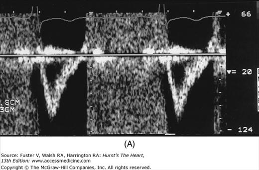
A. PW Doppler tracing from a patient with aortic regurgitation. The transducer is in the apical position and the sample volume is in the left ventricular outflow tract. A laminar envelope is seen during systole, whereas aliased flow is present during diastole because of high-velocity flow. B. CW Doppler tracing through the left ventricular outflow tract (with transducer in the apical position). The maximal velocity of the aortic regurgitation is now measurable, but all other velocities along the Doppler beam are recorded as well. CW, continuous wave; PW, pulsed wave.

The problem of range ambiguity can be overcome by pulsed-wave Doppler (PWD). Short bursts of signal are transmitted from the transducer at a given pulse repetition frequency (PRF). The instrument then receives the signal for only a brief period: an interval that corresponds to the time required for sound energy to travel and return from a specific site along the beam path. The operator selects the location at which flow is to be examined by positioning a sample volume, and the instrument determines the period during which to receive the incoming reflected frequencies. With PWD only a single piezoelectric crystal is needed, and flow can be recorded in one small area within the heart or vasculature.46 Unfortunately, pulsed Doppler techniques use intermittent sampling and are therefore susceptible to a problem of range ambiguity referred to as aliasing.50 Aliasing is the erroneous representation of flow in the direction opposite to that in which it is actually occurring. To correctly record the velocity of blood flow by pulsed Doppler, the PRF must be at least double the Doppler shift frequency, a value known as the Nyquist limit. If the blood flow examined is of very high velocity or far from the transducer (requiring a long transit time), it may necessitate an unobtainably high PRF. In such cases, aliasing will occur as Doppler signals that depict flow at high velocity in ambiguous or opposite directions compared with actual flow (see Fig. 18–28A). An intermediate-mode, high-PRF Doppler is also available. This mode enables higher velocity recordings to be obtained at a compromise of depicting several sample sites simultaneously.
The major limitation of pulsed and CW Doppler (spectral Doppler) is that no spatial information regarding the size, shape, and 2D direction of flow is provided. An extension of PWD techniques, color-flow Doppler (CFD), provides real-time M-mode or 2D imaging of blood flow by presenting the velocity and direction of RBC movement as shades of color superimposed on gray-level 2D tissue structure. Standard pulsed Doppler yields flow signals from a single site along a single scan line. In CFD, rapid pulsed-wave interrogations are performed at multiple sites for multiple scan lines to create a spatially correct and dynamic display of moving blood within the heart and vasculature (Fig. 18–29). Doppler signals are presented as colors assigned to individual sites (Fig. 18–30). Blood flow moving toward the transducer is displayed in red, flow away from the transducer is displayed in blue, and increasing velocity is depicted in brighter shades of each color. The variance within each signal is calculated as a statistical marker of turbulence and is presented by adding green to the image (Fig. 18–31). Therefore, turbulent flow jets appear as a mosaic mix of colors. CFD also can be superimposed onto M-mode tracings (Fig. 18–32), often termed Color M-mode imaging, and is helpful in clarifying the timing of flow phenomena.
Figure 18–32
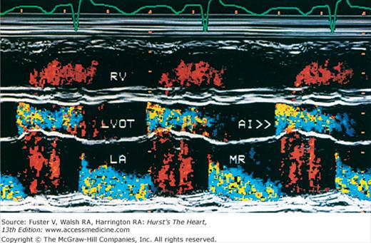
Color-flow Doppler superimposed on an M-mode image. The transducer is in parasternal position, and the cursor is directed through the left ventricular outflow tract (LVOT) and left atrium (LA). The patient under study has both aortic insufficiency (AI) and mitral regurgitation (MR). RV, right ventricle.
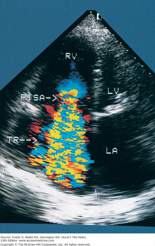
Figure 18–30


Apical four-chamber images with color-flow Doppler during diastole (A) and systole (B). Red flow indicates movement toward the transducer (diastolic filling); blue flow indicates movement away from the transducer (systolic ejection). LV, left ventricle; RA, right atrium; RV, right ventricle.
Figure 18–29
Simplified mechanism of color-flow Doppler imaging. Single-gate (left) or multiple-gate pulsed Doppler (center) can evaluate flow at points along a single ultrasound beam path. Color-flow imaging (right) assesses the velocity and direction of flow for multiple sample volumes along multiple beam paths and assigns a color indicative of velocity and direction at each sample volume site. Reproduced with permission from Hagan AD, DeMaria AN. Clinical Applications of Two-Dimensional Echocardiography and Cardiac Doppler. Boston, MA: Little, Brown; 1989.
Normal flow is laminar, with all RBCs exhibiting the same velocity and direction of flow. Most pathologic conditions, with the exception of atrial septal defects, involve disturbed or turbulent flow and share a common hydrodynamic basis for the resultant flow dynamics. Specifically, nearly all circulatory disturbances (stenosis, regurgitation, shunt) involve blood flow from a high-pressure chamber to a lower pressure chamber through a restricted orifice.45 For example, aortic stenosis (AS) is a forward flow disturbance in which turbulent blood travels from a high-pressure LV to a lower pressure aorta through a restricted aortic orifice in systole. Aortic regurgitation (AR) is a retrograde flow disturbance in which turbulent blood regurgitates from a high-pressure aorta to a lower pressure left ventricle through a small regurgitant orifice in diastole. In each case, the pressure gradient results in a high-velocity jet coursing through a restricted orifice, reaching its maximal velocity at a site just distal to the orifice, designated the vena contracta, at which time shear forces produce vortices resulting in flow of varying direction and velocity (Fig. 18–33). In each case, the velocity of the jet is related to the pressure gradient across the orifice. On pulsed Doppler recordings, these hemodynamic abnormalities cause broadening of the spectral signal and aliasing. On CW recordings, high velocity represents the primary abnormality. By color-flow imaging, the disturbance is manifest by the increased variance and higher velocities in the signal.
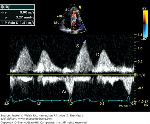
A clinical Doppler examination must be performed with full consideration of the different Doppler modalities available, the types of information each can provide, the multiple sites for flow interrogation, and the spectrum of pathologic lesions that produce flow disturbances. However, most echocardiographic examinations include screening for flow disturbances by CFD. Because Doppler signals are best recorded with the ultrasound beam parallel to flow, screening is typically performed in long-axis or apical views. Any flow disturbances visualized are subsequently examined by CW spectral recordings and, in most laboratories, by PWD. Although CW examination is typically reserved for flow disturbances, PWD may also be of value in quantifying flow dynamics in the setting of laminar flow. In this regard pulsed Doppler recordings obtained at the mitral, tricuspid, and aortic valvular orifices, PA, and pulmonary veins constitute part of a standard echocardiogram (see Figs. 18–26, 18–34 to 18–37). Finally, the usual Doppler examination will include tissue Doppler recordings from a region of interest placed in the septal and lateral mitral annulus in the apical four-chamber view.

Because the Doppler examination is usually performed with a long-axis or apical transducer orientation, diastolic filling is characteristically encoded in red and ejection in blue (see Fig. 18–30). Color aliasing is often observed at the levels of the mitral annulus and LV outflow tract as an abrupt change from bright red to bright blue or vice versa, usually in the center of the flow stream. Pulsed Doppler recordings of transmitral flow velocities are often recorded at the level of both the leaflet tips and annulus. Velocities are higher at the tips, whereas recordings at the annulus offer the ability to calculate flow through a cross-sectional area that is relatively uniform throughout the cardiac cycle. A sample volume positioned in the right upper pulmonary vein reveals systolic (S) and diastolic (D) flow velocities of nearly equal magnitude followed by a short, low-velocity reversal of flow into the pulmonary veins after atrial contraction (A) (see Fig. 18–36). Flow in the LV outflow tract is characterized by a progressive increase of velocity peaking in early systole, followed by a more gradual deceleration of flow (see Fig. 18–35). Examinations of the tricuspid and pulmonary valves give qualitatively similar results to those of the mitral and aortic valves (see Figs. 18–26 and 18–37). Normal values for forward flow velocity are given in Table 18–4. Velocity in normal individuals is highest in the aorta and is less than 2 m/s.51 Other common measurements include the acceleration time, from the beginning of flow to peak velocity of flow in the ascending aorta or PA, and the deceleration time, from LV inflow peak E-wave velocity extrapolated to baseline zero velocity.
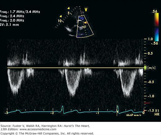
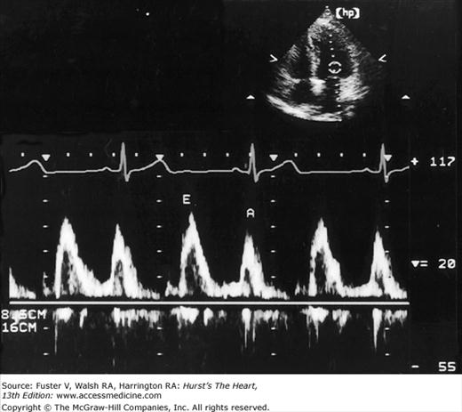
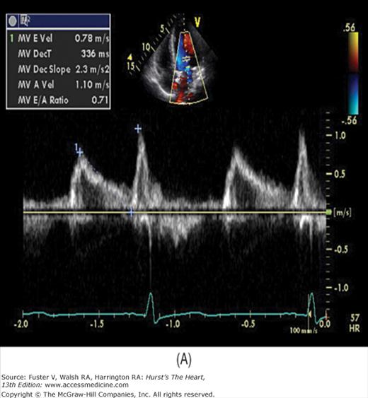
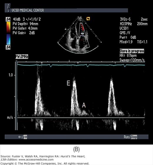
There has been a great deal of interest in using mitral inflow velocity patterns to evaluate LV diastolic properties.52-55 Transmitral filling velocities reflect the pressure gradient between the LA and LV during diastole52 (see Fig. 18–34). In early diastole, pressure in the LV normally falls below that in the LA, producing an increase in velocity due to rapid transmitral inflow (E wave). Flow decelerates as the pressures equilibrate in mid-diastole. In late diastole, LA contraction restores a small gradient, causing transmitral flow to accelerate to a second peak (A wave) that is of less magnitude than the E wave. In individuals in whom early LV relaxation is impaired, the transmitral pressure gradient is blunted, resulting in a decrease in both the velocity of early filling and rate of E-wave deceleration53,54 (Fig. 18–38A). Conversely, in patients with marked increases of LA pressure and LV stiffness, early diastolic filling velocities are high, deceleration is rapid, and late filling after atrial contraction is markedly reduced. This is the so-called restrictive pattern of LV filling (see Fig. 18–38B). Accordingly, an E-wave velocity that is substantially less than the A-wave velocity and is accompanied by a prolonged deceleration time represents evidence of impaired early diastolic relaxation by Doppler, whereas an increased E-wave velocity and decreased A-wave velocity (E/A ratio >2.5:1 or 3:1) accompanied by a diminished deceleration time (<160 ms) is indicative of a noncompliant LV with markedly elevated left atrial pressures.54 A restrictive pattern occurs with restrictive cardiomyopathy or advanced LV dysfunction of any cause and in pericardial disease.56
Figure 18–38

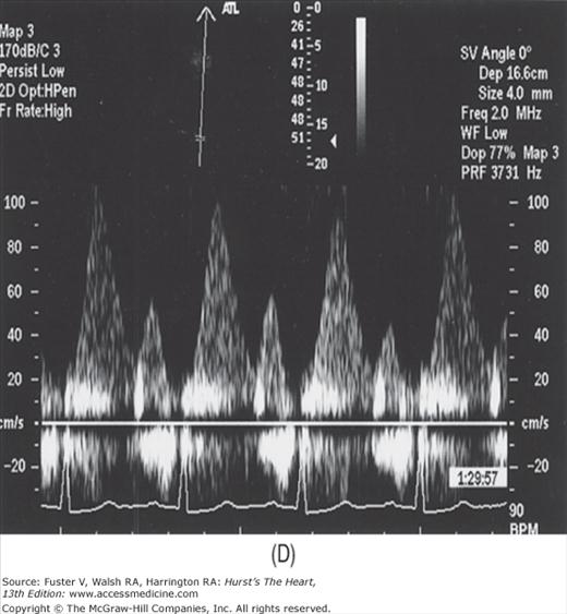

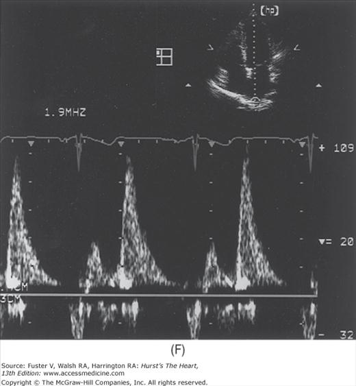
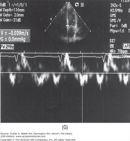
A. Pulsed-wave Doppler (PWD) tracing of diastolic relaxation abnormality (see text for details). B. PWD tracing of diastolic restrictive abnormality (see text for details). (continued)”Figure 18–38. (continued) C. Tissue Doppler recording of normal lateral mitral annular motion (apical transducer position). Peak early diastolic annular velocity is 17 cm/s. D. PWD recording of pulmonary venous flow in mild diastolic dysfunction (abnormal relaxation). The S wave is prominent, whereas the D wave is small. E. Tissue Doppler image (septal mitral annulus) in mild diastolic dysfunction. Early diastolic velocity is blunted (4 cm/s). F. PWD recording of pulmonary venous flow in severe diastolic dysfunction. The S wave is small, whereas the D wave is prominent. G. Tissue Doppler image in severe diastolic dysfunction. Both Em and Am velocities are abnormally low. A, atrial contraction; E, early rapid filling.
These abnormal mitral inflow patterns are often useful in suggesting the presence of and characterizing diastolic dysfunction. Several variables other than diastolic function, however, are capable of influencing transmitral filling velocities. Transmitral Doppler filling dynamics are affected by the age of the patient, changes in heart rate,57 respiration, and even the position of the Doppler sample volume within the MV orifice.58 Transmitral inflow is sensitive to loading conditions, and reductions in LV preload can induce a striking decrease in early transmitral filling velocities independent of changes in diastolic properties. The influence of LV loading on transmitral filling is most striking when an increase in LA pressure caused by cardiac dysfunction obscures impaired relaxation by restoring early diastolic filling velocities, thus inducing pseudonormalization. Therefore, because Doppler transmitral filling dynamics have many limitations in assessing diastolic function, particular filling patterns should not be interpreted as pathognomonic findings of diastolic dysfunction, but rather as components of a complete clinical and echocardiographic evaluation.
The addition of pulsed-wave tissue Doppler imaging (TDI) has significantly enhanced the noninvasive assessment of diastolic function. Although TDI can assess systolic performance, it is most often used to measure the motion of the mitral annulus away from the transducer during diastole. The diastolic pattern is similar to the PW transmitral flow pattern, but the velocities are considerably less and in the opposite direction. The normal velocity of the early TDI motion (Em) is 12 cm/s or greater at the lateral mitral annulus and 8 cm/s or more at the septal mitral annulus. In addition, the ratio of transmitral E velocity to Em is normally in the range of 8 to 12.
In a young, healthy individual, the E/A ratio is generally between 1.5:1 and 2:1 (see Fig. 18–34). Because of high LV compliance, the D velocity is greater than the S velocity in the pulmonary venous Doppler tracing (see Fig. 18–36). With age the LV compliance drops somewhat, so that by age 40 to 50 years, the S and D pulmonary venous velocities are similar. As mentioned, TDI Em velocity is 12 cm/s or greater (see Fig. 18–38C). In the setting of mild diastolic dysfunction, the E/A ratio is <1, the E deceleration time is prolonged (relaxation abnormality; see Fig. 18–38A), and the pulmonary venous S wave is considerably larger than the D wave (S/D ratio >1) (see Fig. 18–38D). TDI shows blunting of the Em wave with relative preservation of the later atrial component (Am) (see Fig. 18–38E).
As diastolic function worsens and LV filling pressures increase, a pseudonormal pattern occurs in the transmitral flow tracing (Fig. 18–39). Pulmonary venous and tissue Doppler imaging are especially helpful in this case: If the S/D ratio is <1 (except in the setting of a young individual), high LV filling pressure is likely present. Similarly, the presence of a low, blunted Em velocity in the setting of a normal transmitral E/A ratio strongly suggests diastolic dysfunction and elevated LV filling pressure. In fact, the ratio of the E/Em velocities correlates reasonably well with pulmonary capillary wedge pressure, and a ratio of >15:1 reliably identifies an abnormal elevation of wedge pressure.59 Of note, the Valsalva maneuver can be helpful in cases of pseudonormal transmitral flow patterns. In normal individuals, both E and A velocities drop to a similar degree with Valsalva. In pseudonormal cases, however, the drop in preload caused by the Valsalva maneuver changes the transmitral pattern to that of mild diastolic dysfunction.
Figure 18–39
Doppler assessment of progressive diastolic dysfunction utilizing transmitral pulsed-wave Doppler, pulmonary venous Doppler, and mitral annular tissue Doppler imaging. A, atrial component of LV filling; Am, myocardial velocity during LV filling produced by atrial contraction; Dec. Time, E wave deceleration time; E, early LV filling velocity; Em, early diastolic myocardial velocity; IVRT, isovolumic relaxation time; PVa, pulmonary vein velocity resulting from atrial contraction; PVd, diastolic pulmonary vein velocity; PVs, systolic pulmonary vein velocity; Sm, systolic myocardial velocity. Reproduced with permission from Zile MR, Brutsaert DL. New concepts in diastolic dysfunction and diastolic heart failure: Part I. Circulation. 2002;105:1387-1393.
In severe diastolic dysfunction, transmitral flow demonstrates a restrictive pattern, with an abnormally high E/A ratio and a markedly shortened E wave deceleration time (see Fig. 18–38B). Concomitant pulmonary venous tracings show a very low S velocity and elevated D velocity (S << D) (see Fig. 18–38F). In some cases, the pulmonary venous atrial reversal wave can be prominent and prolonged. In this regard an abnormally prolonged duration of reversed pulmonary venous flow during atrial contraction accurately predicts elevated LV filling pressures.52 TDI in severe LV diastolic dysfunction shows marked blunting of both Em and Am velocities (see Fig. 18–38G). An exception to this occurs in constrictive pericarditis, where early diastolic mitral annular motion is often preserved. Thus when transmitral and pulmonary venous Doppler suggest severe diastolic dysfunction, a normal TDI pattern suggests constrictive rather than restrictive physiology.
Color M-mode imaging has been used to assess the velocity of propagation of the transmitral filling stream into the LV. This technique appears helpful in distinguishing constrictive pericarditis from restrictive cardiomyopathy.
Many recent studies have demonstrated the importance of LA enlargement in the setting of diastolic dysfunction and elevated LV filling pressure. Indeed, left atrial enlargement appears to predict adverse cardiovascular outcomes in general, not just elevated LV diastolic pressure.60 Clearly, the E/A ratio, pulmonary venous flow pattern, and mitral annular TDI are all load dependent and can often change quickly with medical intervention. However, LA volume increases over the long term in response to elevated pressure.61 LA volume does not change significantly with short-term fluctuations in loading conditions. LA volume can be calculated relatively easily and should be normalized to body-surface area. LA volume >28 cc/m2 is abnormal and signifies long-term diastolic dysfunction and elevated LV filling pressure.61 An exception to this relationship occurs with atrial fibrillation: In this setting, LA volume is less predictive of cardiovascular events and elevated LV filling pressure.60
Doppler interrogation provides a unique and complementary noninvasive assessment of systolic function. Thus LV systolic dysfunction often results in decreased aortic velocity and acceleration time. As discussed below, in the presence of mitral regurgitation (MR), the acceleration of the MR jet can provide information regarding contractile function.62
One of the most important applications of Doppler is in the calculation of the stroke volume.63 The volume of flow through any orifice or tube can be calculated as the product of the cross-sectional area through which flow occurs and the velocity of that flow (Fig. 18–40). Measurements of anatomic cross-sectional area can be derived from echocardiographic images, whereas velocity can be determined by Doppler. As the annulus of the aortic valve is nearly circular, its cross-sectional area can be estimated from a measurement of diameter as π (diameter/2)2. The PWD envelope also can be recorded at the same level. The mean flow velocity through the orifice is calculated by integrating velocity over time (that is, by measuring the area under the Doppler curve). This velocity-time integral, often called the stroke distance, is then multiplied by the cross-sectional area at the level of the Doppler interrogation to obtain the stroke volume.63,64 The product of the stroke volume and heart rate then yields cardiac output.
Figure 18–40
Calculation of stroke volume. Multiplying the cross-sectional area (CSA) of the blood column in the ascending aorta by the distance the column moves during a single cardiac contraction yields the stroke volume (SV). The velocity-time integral (VTI), expressed in units of length, represents the stroke distance. Modified with permission from Pearlman AS. Technique of Doppler and color flow Doppler in the evaluation of cardiac disorders and function. In: Schlant RC, Alexander RW, eds. The Heart, Arteries, and Veins. 8th ed. New York, NY: McGraw-Hill; 1994:2229.
Calculation of stroke volume by the Doppler method involves a number of assumptions. The orifice must be circular and constant in size, and the flow velocity must be uniform throughout the cross-sectional area. In addition, the angle between flow and the interrogating beam must be <20 degrees. Nevertheless, Doppler-derived measurements of cardiac output and stroke volume have been shown to correspond well with thermodilution, Fick, and angiographic calculations, but the correlation is not perfect.63,64
Theoretically, stroke volume can be calculated at any valve annulus.64 In clinical practice, however, this is not always possible. Because the measurement of annular radius is squared in the computation of area, it is the most important source of error of Doppler stroke-volume analyses. Stroke-volume analysis through the mitral annulus is cumbersome; it is uncertain whether the mitral annulus is best described as a circle or an ellipse, and the cross-sectional area of the annulus probably changes slightly during diastole. Despite these limitations, measurements of stroke volume through the various cardiac valves are clinically useful and can be used to calculate pulmonary-to-systemic shunt ratios, regurgitant volumes,65,66 and orifice areas of stenotic valves by the continuity equation.67
An important application of Doppler echocardiography is the calculation of pressure gradients within the cardiovascular system using a modification of the Bernoulli equation.68 This theorem states that the pressure drop across a discrete stenosis in the heart or vasculature occurs because of energy loss caused by three processes: (1) acceleration of blood through the orifice (convective acceleration), (2) inertial forces (flow acceleration), and (3) resistance to flow at the interfaces between blood and the orifice (viscous friction). Therefore, the pressure drop across any orifice can be calculated as the sum of these three variables (Fig. 18–41). The pressure gradient can be calculated from the velocities of blood proximal to and at the level of an orifice:
Figure 18–41
The modified Bernoulli equation. Pressure drop across a small orifice can be estimated as four times the square of the peak velocity (if the proximal velocity is <1 m/s). V1 and P1, proximal velocity and pressure; V2 and P2, distal velocity and pressure. Modified with permission from Pearlman AS. Technique of Doppler and color flow Doppler in the evaluation of cardiac disorders and function. In: Schlant RC, Alexander RW, eds. The Heart, Arteries, and Veins. 8th ed. New York, NY: McGraw-Hill; 1994:2229.
Gradient = 4[(orifice velocity)2 − (proximal velocity)2]
If the blood velocity proximal to the stenosis is low (<1.0 m/s), this term can be ignored. The resulting modified equation states that the pressure gradient across a discrete orifice is equal to four times the square of the peak velocity (V) through the stenosis (PG = 4V2).68
The modified Bernoulli equation can be used to calculate pressure gradients across any flow-limiting orifice and has been validated against invasive measurements.69 If at least trivial valvular regurgitation is present, systolic gradients across the tricuspid valve and end-diastolic gradients across the pulmonic valve can be calculated.70 If the RV diastolic pressure is known (or estimated as the right atrial or central venous pressure), peak RV and PA pressure (assuming pulmonic stenosis is absent) can be computed as follows:71
Peak PA pressure = 4(TR velocity)2 + RA pressure
End-diastolic PA pressure (PAD) also can be calculated:
PAD = 4(end-diastolic pulmonary regurgitation velocity)2 + RA pressure
In the presence of MR, a variety of calculations can be made. With measurement of peak systolic arterial pressure, systolic left atrial pressure can be estimated:
LA systolic pressure = systolic blood pressure − 4(MR velocity)2
Further, the acceleration of the MR jet can be used to estimate LV systolic dP/dt. From the Bernoulli equation, the LA-to-LV pressure gradients at regurgitant velocities of 1 and 3 m/s are 4 and 36 mm Hg, respectively. Therefore, dP/dt can be calculated as 32 mm Hg divided by the time (in seconds) required for the mitral regurgitant jet to accelerate from 1 to 3 m/s. In the case of ventricular septal defects (VSDs) or aortopulmonary shunts, measurements of the peak systolic arterial pressure and the peak Doppler velocity across the defect allows calculation of the RV (or pulmonary arterial) systolic pressure.
Although transvalvular pressure gradients can be calculated from CW Doppler recordings using the modified Bernoulli equation, gradients sometimes can be misleading in the evaluation of valvular stenosis. The transvalvular gradient is determined by both the size of the stenotic orifice and the stroke volume traversing it. Severe AS and accompanying LV systolic dysfunction may produce a low transvalvular gradient despite a small valve area, whereas coexistent AR may result in a large gradient with only mild AS. The calculation of orifice area by Doppler echocardiography uses the continuity equation, which is derived from the law of the conservation of mass and states that the product of cross-sectional area and velocity is constant in a closed system of flow (Fig. 18–42). Thus in the case of AS, the product of the area and velocity of the left LV outflow tract equals the product of the area and velocity of the aortic valve orifice. Measurements of annular diameter and integrated velocity are derived by the standard volumetric approach, whereas the velocity across the stenotic orifice is derived by CW Doppler. The equation is then solved for the valve area.67
Figure 18–42
The continuity equation. In a closed system (top) with constant flow, Q1 = Q2. Therefore, A1 × V1 must equal A2 × V2. Determination of any three of the variables allows calculation of the fourth. Clinically (bottom), the area of the left ventricular outflow tract (LVOT) can be estimated and used to determine AV area. AV, aortic valve. Reproduced with permission from Hagan AD, DeMaria AN. Clinical Applications of Two-Dimensional Echocardiography and Cardiac Doppler. Boston, MA: Little, Brown; 1989.
The most common pitfall is an inaccurate estimation of the cross-sectional area proximal to the stenosis. In addition, it is essential that blood velocity proximal to a stenosis be measured outside the area of flow acceleration. Finally, the continuity equation actually solves for the area of the vena contracta, which is usually just distal to the stenotic orifice. In general, however, this correlates well with the aortic valve area.
Although CFD yields primarily qualitative information, it is unique in its ability to provide measurements of the size of flow disturbances. The size of a turbulent jet should correlate with the volume of blood contained within the flow disturbance. Regardless of the lesion, however, the area of turbulence recorded by CFD has multiple determinants.72 The pressure gradient operative in any flow disturbance is also an important determinant of the spatial distribution or spray area of turbulence.72 Also, the size of a flow disturbance is influenced by the orifice through which flow occurs, as well as the size and compliance of the receiving chamber.72 Finally, a number of technical factors can influence jet size, including instrument gain, the angle of incidence of the interrogating beam, the frequency and pulse repetition rate of the transducer, and the temporal sampling rate.73 Therefore, measurements derived from the size of the turbulent jet recorded by color Doppler are at best semiquantitative and should not be expected to correlate with the volume of blood contained in the flow disturbance.
Transesophageal Echocardiography
Transthoracic echocardiography (TTE) usually defines cardiac anatomy and function satisfactorily, often obviating the need for further cardiac imaging. Occasionally, however, TTE does not provide complete or adequately detailed information. This is especially true in the evaluation of posterior cardiac structures (eg, LA, LA appendage, interatrial septum, aorta distal to the root), in the assessment of prosthetic cardiac valves, and in the delineation of cardiac structures <3 mm in size (eg, small vegetations or thrombi). Ultrasonic imaging from the esophagus is uniquely suited to these situations, because the esophagus is adjacent to the LA and the thoracic aorta for much of its course74 and affords excellent access of the interrogating beam to these structures.
Flexible transesophageal ultrasound probes capable of multiplanar imaging of the heart and full pulsed-wave, CW, and CFD capabilities quickly supplanted the original biplane probes.75 The latest generation of transesophageal echocardiography (TEE) transducers provides for real-time 3D imaging.
Although images can be recorded from a variety of probe positions, most authorities recommend three basic positions: (1) posterior to the base of the heart, (2) posterior to the LA, and (3) inferior to the heart (transgastric position) (Fig. 18–43). Figures 18–44 through 18–47 show TEE images obtained in various planes through the heart. It must be emphasized that, with the transducer in the esophagus, posterior structures appear at the top of the image. With the transducer in the stomach, a short-axis view is standardly obtained, with long-axis and apical views available to a variable degree. On withdrawing the transducer to the esophagus, apical-equivalent four-chamber and long-axis views with multiple intermediate projections are usually obtained. Further withdrawal of the probe to the base yields excellent views of the atria, great vessels and semilunar valves, and pulmonary veins. Of particular value are views that delineate the LA appendage, all three leaflets of the aortic valve in short axis, and the transverse and descending aorta.

Figure 18–46
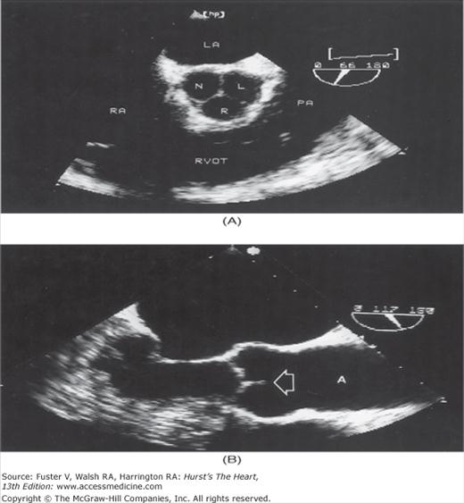
A. Modified short-axis view through the level of the AoV, demonstrating the left (L), right (R), and noncoronary (N) valvular cusps. B. Magnified longitudinal view of the AoV (arrow) showing the coaptation of the cusps and the sinuses of Valsalva. C. Longitudinal image at level of the aortic arch, demonstrating the transverse aorta (A), the brachiocephalic vein (V), and the main pulmonary artery (PA). The pulmonic valve is visible as well (arrow). Ao, aorta; AoV, aortic valve; LA, left atrium; PA, pulmonary artery; RA, right atrium; RVOT, right ventricular outflow tract. B, reproduced with permission from Blanchard et al.74
Figure 18–47
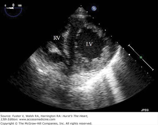
Short-axis transesophageal echocardiography plane through the left ventricle from transgastric position. The inferior wall is closest to the transducer, the anterior wall farthest. The interventricular septum is to the reader’s left, the lateral wall to the right. LV, left ventricle; RV, right ventricle.
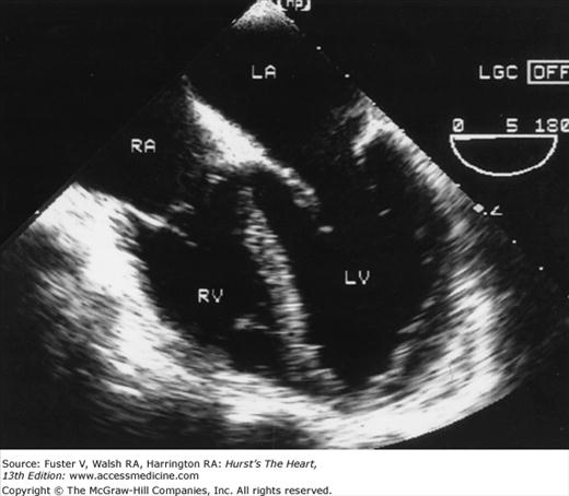
TEE is an important imaging modality for the diagnosis and management of infective endocarditis and its complications, including valvular vegetations, chordal rupture, fistulas, perivalvular abscesses, and mycotic aneurysms.76 TEE is more accurate in detecting vegetations, valve perforations, and abscesses than TTE76 and provides prognostic information as well (Fig. 18–48). In addition, TEE imaging may aid in accurate quantification of valvular disease (particularly MR) if TTE is inconclusive (Fig. 18–49). TEE is especially useful for Doppler interrogation of the pulmonary veins (Fig. 18–50). Flow patterns in these vessels reflect LA pressure, and systolic reversal of pulmonary venous flow is an accurate marker of severe MR.77 Although MR color jets are easier to see with TEE than TTE, they are usually larger, and care must be exercised not to overestimate the severity of the regurgitation. Multiplane TEE can be used to planimeter the orifice area in AS.78 The technique is also quite helpful in detection of aortic disease, including dissection, aneurysm, congenital malformations, and atherosclerosis.74 Because of its portability, accuracy, and short preparation and procedural times, TEE is the recommended diagnostic study in many cases of suspected aortic dissection, particularly in unstable patients. (Fig. 18–51).74,79
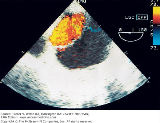
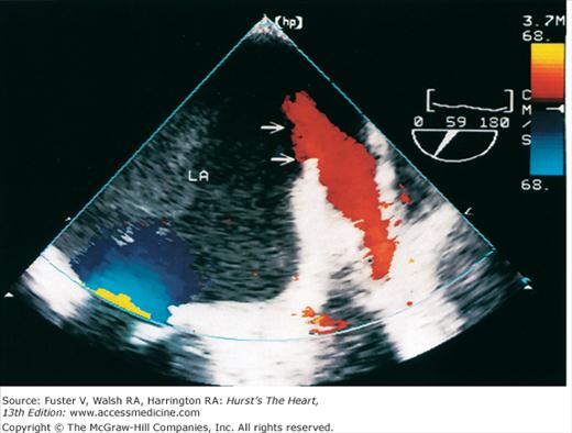
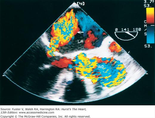
Figure 18–48
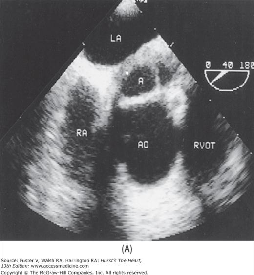
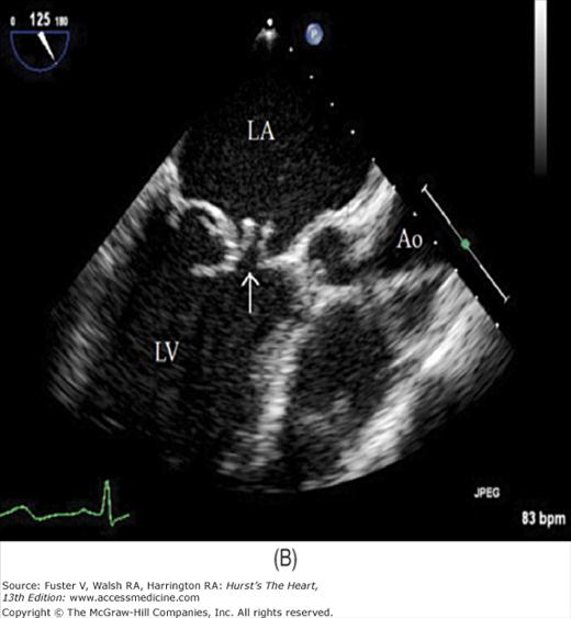
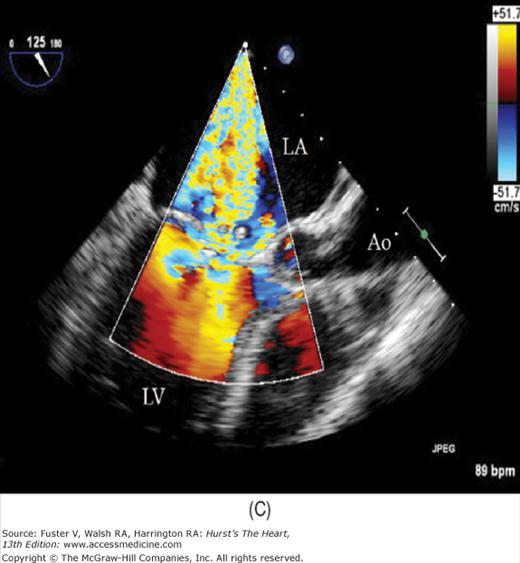
A. Short-axis transesophageal echocardiography (TEE) plane through the cardiac base. A large septated abscess cavity (A) is present between the aortic root (AO) and the left atrium (LA). B. Modified three-chamber TEE plane showing perforation of the anterior mitral valve leaflet (arrow) in a case of endocarditis. C. Color imaging reveals severe mitral regurgitation. LA, left atrium; LV, left ventricle; Ao, aorta.
Thromboemboli may originate from posterior cardiac structures such as the LA and LA appendage, interatrial septum, and aorta80; therefore, TEE has received wide application in the evaluation of possible cardiogenic embolization. The ability of TEE to visualize the LA appendage is of particular value (Fig. 18–52). TEE can also detect spontaneous contrast signals, which appear to represent transient rouleaux formation and predispose to thromboemboli. In addition, TEE has provided unique real-time images of mobile, pedunculated, atherosclerotic debris in the thoracic aorta (Fig. 18–53). Although the optimal therapy for this disorder is currently unknown, warfarin may be helpful, and mobile or protruding aortic atheromas appear to be significant risk factors for embolic events.81,82
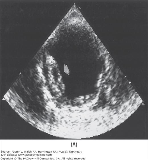
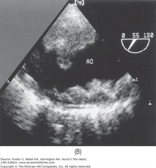

Another proven application of TEE is the evaluation of prosthetic valve dysfunction, particularly mechanical valves in the mitral position.83 The areas behind prosthetic valves are usually hidden from view when transthoracic imaging is used. TEE is clearly superior to TTE imaging for detection of prosthetic regurgitation, infection, tissue ingrowth, and thrombosis (Fig. 18–54).
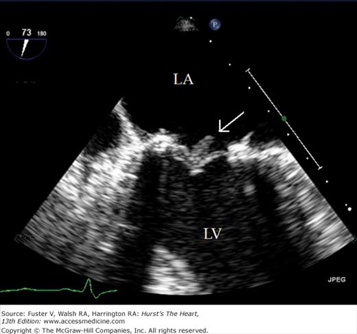
TEE has also become an important intraoperative tool for the detection of cardiac ischemia, the evaluation of valve function after repair or replacement, and the delineation of CHD. Cardiac surgeons often rely on intraoperative TEE for evaluation of cardiac anatomy and confirmation of a success of surgical repair before closing the chest. In this regard, TEE has almost completely replaced TTE. When TTE images are inadequate, TEE helps manage critically ill patients and also can be used to monitor or guide interventional procedures, such as transseptal catheterization, mitral valvuloplasty, pericardiocentesis, and endomyocardial biopsy. The use of real-time 3D echo has proven of great value in examining mitral leaflet and annular anatomy and function in patients with mitral valve disease, as well as in guiding the deployment of devices, such as for atrial septal closure.


