Transthoracic echocardiography is a reliable and versatile tool for the assessment of cardiac structure, function, and hemodynamics. It has advantages over other cardiovascular imaging modalities in that it is relatively inexpensive, does not incur radiation exposure to the patient, is noninvasive, displays live real-time images, and is widely available. Common indications and corresponding aims of the echocardiographic evaluation are listed in Table 67.1.
II. BASIC PRINCIPLES OF ECHOCARDIOGRAPHY.
Sound waves consist of mechanical vibrations that produce alternating compressions and rarefactions of the medium through which they travel. Ultrasound consists of sound waves in the frequency range that is higher than what is audible by humans (> 20,000 Hz). All waves can be described by their frequency (f), wavelength (λ), velocity of propagation (v), and amplitude. The velocity of ultrasound in soft tissue (e.g., myocardium and blood) is 1,540 m/s. Frequency is defined by the number of cycles occurring per second (cycles/second or Hz) and wavelength is measured in meters (m). Velocity, frequency, and wavelength are described by the following relationship:
The typical adult echocardiographic examination uses a transducer with ultrasound frequency between 2.5 and 3.5 million Hertz (MHz). Based on the equation above, a 3-MHz transducer results in an ultrasound wavelength of approximately 0.50 mm. This has important implications since image resolution cannot be > 1 to 2 wavelengths (e.g., 1 mm with a 3-MHz transducer). In addition, the depth of penetration of the ultrasound wave is directly related to the wavelength, with shorter wavelengths penetrating a shorter distance. Therefore, higher frequency transducers result in the use of shorter wavelengths that improve image resolution but at the cost of reduced depth penetration.
Transducers use a piezoelectric crystal to generate and receive ultrasound waves. A piezoelectric substance has the property of changing its size and shape when an electric current is applied to it. An alternating electrical current will result in rapid expansions and compressions of the material and thus produce an ultrasound wave. The piezoelectric crystal also deforms in shape when an ultrasound wave strikes the material, resulting in the production of an electric current. The transducer, and the piezoelectric crystal, thus oscillates between a short burst of transmitting ultrasound waves, with a brief period of no ultrasound transmission when it awaits reception of the reflected signals.
Tissue harmonic imaging has become the standard imaging technique in many laboratories. It utilizes the principle that as ultrasound waves propagate through tissue, the waveform becomes altered by the tissue, with the generation of new waveforms of higher frequency but which are multiples of the baseline fundamental frequency. Setting the transducer to receive only harmonic sound waves that are multiples of the fundamental frequency improves image quality significantly. This image quality improvement is based on the fact that weak signals, which tend to be artifacts, create almost no harmonics. In addition, shallow structures, such as the chest wall, generate weak harmonic signals, whereas at depths of 4 to 8 cm, where the heart is located, maximal harmonic frequencies develop. These phenomena result in fewer near-field artifacts and better endocardial definition. One limitation of harmonic imaging is that valve leaflets appear thicker—an artifact generated during image processing that appears to be related to the rapid motion of the leaflets.
TABLE 67.1 Common Indications and Corresponding Aims of Echocardiographic Evaluation
Indications
Echocardiographic evaluation
Valvular heart disease
Valve morphology, regurgitation and/or stenosis severity and etiology, and ventricular size and function
Infective endocarditis
Vegetation, abscess, fistula, valvular function, and ventricular size and function
Coronary artery disease
Wall motion abnormalities, ventricular function, and mitral regurgitation/ventricular septal defect and other ischemic complications
Congestive heart failure
Systolic function, wall motion abnormalities, chamber size, valvular pathology, and diastolic function
Pericardial disease
Pericardial effusion, pericardial thickening ± calcification, and RV size and function
Cardiac tamponade
Pericardial effusion; RA diastolic collapse; RV early diastolic collapse; respiratory variations in mitral, tricuspid pulmonary venous, and hepatic venous flow; and IVC size and respiratory variation
Ascending aortic pathology
Aneurysm, atheroma, dissection or intramural hematoma, and aortic valve pathology
Pulmonary hypertension
RV systolic pressure, RV and LV function, and tricuspid, pulmonary, and mitral valve pathology
Interatrial shunt and respiratory effects on IVC diameter
Systemic hypertension
LV function, LV wall thickness, and evidence of aortic coarctation
Embolic disease
LA and LV thrombus, mitral valve pathology, aortic atheroma, LV function, and interatrial shunt
Arrhythmias
LA and LV thrombus, ventricular size and function, atrial dimensions, and mitral valve pathology
Syncope
LV outflow tract obstruction, aortic and mitral valve pathology, LV function, and congenital abnormalities
Cardiac trauma
Ascending aortic dissection, ascending aortic aneurysm, and cardiac tamponade
Congenital heart disease
Congenital anomaly and shunt calculation
Critical illness
LV function, valvular pathology, pericardial effusion/tamponade, right-to-left shunt, and volume status
IVC, inferior vena cava; LA, left atrial; LV, left ventricular; RA, right atrial; R V, right ventricular.
The steps involved in creating a final ultrasound image are transmission and reception of waves, conversion to electrical signals, filtering, and extensive computer processing. The details of image processing, formation of artifacts, advanced physics, and technical aspects of echocardiography are beyond the scope of this chapter, but these are briefly discussed in Section VII.
Patient and probe positioning, electrocardiographic lead placement, and transducer selection are the first steps to beginning the echocardiographic examination.
A. Patient and probe positioning.
The probe can be held with the right or left hand depending on the patient side that one chooses to scan from. For the parasternal and apical positions, the patient should be in the left lateral decubitus position, with the left arm extended behind the head, as this brings the heart into contact with the chest wall. The subcostal and suprasternal views require the patient to be in the supine position.
B. Electrocardiographic lead placement.
The ECG allows identification of arrhyth mias and timing of cardiac events during the echocardiographic examination, and it is used as a timing marker for digital recording of images. Typically, digital “clips” are set to record a predefined number of cardiac cycles (usually one but sometimes two), with timing based on the ECG. It is important that irregular beats be identified and excluded from the analysis. For example, a postectopic beat will falsely increase the two-dimensional (2D) assessment of ejection fraction (EF) and the Doppler assess ment of transaortic gradient. In general, any Doppler index requires the average of at least three measurements. For patients in atrial fibrillation, 7 to 10 beats should be averaged. For patients with very high heart rates, or with a noisy electrocardiographic signal, the digital clips can be set to record for a predefined period of time (usually 2 seconds).
C. Transducer selection.
The adult echocardiographic examination typically begins with a 2.5- to 3.5-MHz phased array transducer. Transducer frequency is important, as at higher frequencies spatial resolution improves but at the expense of reduced depth penetration. Higher frequency (3.0 to 5.0 MHz) transducers may be used in thin or pediatric patients or intraoperatively for epiaortic scanning. Therefore, for optimal 2D resolution, select the highest frequency transducer that will provide adequate far-field penetration.
With regard to transducer frequency for the Doppler examination, lower frequency transducers can record higher velocities (see Doppler equation later in the chapter). The Pedoff probe is a continuous-wave (CW), nonimaging probe (typical frequency being 1.8 MHz) used mainly to detect higher velocity profiles and confirm velocities obtained by other imaging methods.
III. IMAGING MODALITES IN STANDARD ECHOCARDIOGRAMS
A. M-mode.
Prior to 2D imaging, the echocardiogram was obtained when the transducer sent an ultrasound wave along a single line and then displayed the amplitude of reflected signal as well as the depth of that signal on an oscilloscope. This was called an A-mode echocardiography. When these line-of-sight ultrasound images were plotted with respect to time, “motion” mode, or M-mode, was produced. Despite the increasing emphasis on 2D imaging, the M-mode display remains a complementary element of the transthoracic examination. Its high sampling rate of approximately 1,800/s, compared with 30/s for 2D echocardiography, provides excellent temporal resolution, and thus it is very useful in the timing of subtle cardiac events that can be missed by the naked eye in 2D imaging. Rapidly moving structures such as the aortic valve, mitral valve, and endocardium have characteristic movements in M-mode. Deviations from these, such as diastolic fluttering of the mitral valve in aortic regurgitation (AR) and systolic aortic valve notching in dynamic left ventricular outflow tract (LVOT) obstruction, may be the only way to detect underlying dysfunction when they are not appreciated in other imaging modalities. M-mode also has a great spatial resolution along the single line and can be used for precise size measurements such as ventricular dimensions in systole and diastole. The M-mode image is displayed like a graph, with time on thex-axis and distance from the transducer on they-axis, with the structures closest to the transducer at the top of the image. In order to align the line of sight accurately, 2D imaging should be used to position the M-mode cursor through the structures of interest.
B. Two-dimensional imaging.
Two-dimensional imaging provides the tomographic views that are envisioned when one thinks of a transthoracic echocardiogram. It not only provides various 2D planes of cardiac structures but also acts as the platform that guides the M-mode and Doppler portions of the examination.
The 2D echocardiographic image is essentially the scan line from M-mode that, instead of having a fixed line of sight, is swept back and forth across an arc. After complex manipulation of the data received by the transducer from the multiple scan lines, a 2D tomographic image is generated for display.
Depending on the depth of the image, a finite amount of time is needed for each scan line to be sent and received by the transducer. As opposed to M-mode that has only one scan line and can provide over 2,000 frames/s, 2D echocardiographic imaging can utilize 128 scan lines but at the expense of a lower rate of 30 frames/s. Faster frame rates can be obtained by electronic manipulation using parallel processing on current ultrasound machines. Doppler overlay of the 2D image tends to slow down the frame rate. This reduction in temporal resolution reinforces the need for M-mode to complement 2D imaging in echocardiography, especially for rapidly moving structures and in precise timing of events.
C. Doppler echocardiography.
The introduction of Doppler technique to echocardiography not only added new imaging capabilities but also transformed echocardiography into a modality that could provide hemodynamic assessment of the heart. Echocardiography has now become the preferred method, and in some cases the gold standard, over cardiac catheterization for certain hemodynamic assessments.
1. Doppler principles.
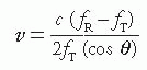
The Doppler principle states that sound frequency increases as the sound source moves toward the observer and decreases as the source moves away. The change in frequency between the transmitted sound and the reflected sound is termed the Doppler shift. This phenomenon is appreciated daily when an ambulance’s siren becomes higher pitched, due to the increase in wave frequency, as it approaches the observer and then lower pitched once it has passed. This Doppler frequency shift directly relates to the velocity of the red blood cell by the following Doppler equation:
where v = velocity, fR = frequency received, fT = frequency transmitted, c = speed of sound in blood (1,540 m/s), and θ = angle between moving object and ultrasound beam.
The cos θ in the Doppler equation makes the calculation of velocity depending on the angle between the beam and the moving structure (red blood cell). Echocardiography machines do not typically incorporate the angle for calculating the resultant velocity, and thus the goal is to have the angle between the ultrasound beam and the blood flow jet of interest to be as close to zero as possible (cos 0 = 1). When this is not possible, the angle should be < 20°, so that the true flow velocity is underestimated by < 6% (cos 20 = 0.94). Adhering to this requirement sometimes mandates off-axis or unusual 2D images to align the Doppler ultrasound signal with desired target. Reference Doppler velocities in the adult examination are given in Table 67.2.
TABLE 67.2 Normal Echo Dimensions in Adults
Factor
Ref. range (cm)
Factor
Ref. range (cm)
(i) Parasternal long axis (M-mode or 2D)
LV end-diastolic diameter
3.5-5.7
LV end-systolic diameter
2.3-4.0
Septal thickness (ED)
0.6-1.1
Posterior wall thickness (ED)
0.6-1.1
Aortic root (ED—M-mode)
2.0-3.7
Left atrium (ES)
1.9-4.0
RV end-diastolic diameter
1.9-3.8
Aortic annulus (systole—2D)
1.4-2.6
Midascending (2D)
2.1-3.4
(ii) Four-chamber view
LV volume (ED) (cm3)
96-157
LV volume (ES) (cm3)
33-68
Ejection fraction (%)
59 ± 6
Left atrial area (cm2)
< 20
(iii) Doppler velocities
Mitral E wave (< 50 y) (cm/s)
72 ± 14
Mitral E wave (> 50 y) (cm/s)
62 ± 14
Mitral A wave (< 50 y) (cm/s)
40 ± 10
Mitral A wave (> 50 y) (cm/s)
59 ± 14
Deceleration time (ms)
140-210
Ascending aorta (m/s)
1.0-1.7
LV outflow tract (m/s)
0.7-1.1
Pulmonary artery (m/s)
0.5-1.3
Pulmonary vein S wave (cm/s)
56 ± 13
Pulmonary vein D wave (cm/s)
44 ± 16
Pulmonary vein A reversal (cm/s)
32 ± 7
ED, end-diastole; ES, end-systole; LV, left ventricular; R V, right ventricular.
2. Spectral analysis
is the term used to describe the way in which pulsed-wave (PW) Doppler and CW Doppler are displayed. By convention, the horizontal axis reflects time and is placed in the middle of the screen with upward deflections representing frequency shifts toward the transducer and downward deflections for frequency shifts away from the transducer. The vertical axis represents the blood flow velocity (or frequency shifts), with the density of pixels on a gray scale reflecting the amplitude of the signal. The final result is that at each time-point the spectral analysis shows blood flow direction, velocity/frequency shift, and signal amplitude.
a. PW Doppler. The purpose of PW Doppler mode is to measure the Doppler shift, and thus velocity, at a specific location of interest within a small sample volume (e.g., mitral inflow velocity at the mitral valve leaflet tips, systolic velocity at the LVOT, and blood flow within the pulmonary veins). In this mode, a single crystal sends short bursts of ultrasound waves at a specific pulse repetition frequency (PRF) to a specific location, which are reflected from moving blood cells at this location and received by the same crystal. The maximal velocity that can be measured is limited by the time required to transmit and receive the ultrasound wave. This is called the Nyquist limit (one-half of the PRF). If a velocity greater than the Nyquist limit is measured, the signal appears as a wrap around the baseline, known as signal aliasing. Hence, the peak velocity is limited by the depth of the area of interest and also by the transducer frequency (inverse relationship according to the Doppler equation; see previous text). PW Doppler has excellent spatial/depth resolution, but it has limited capacity to measure high velocities due to the Nyquist limit. It is, therefore, used primarily to measure low-velocity flow (< 2 m/s) at specific sites in the heart.
b. CW Doppler. CW Doppler employs two crystals, one continuously send ing ultrasound waves and the other continuously receiving the waves. It measures Doppler shift along the entire beam, rather than at a specific location. Unlike PW Doppler, CW Doppler measures the maximal velocity along the entire ultrasound beam but it does not localize the precise posi tion of that peak velocity. However, this is often apparent anatomically or can be deduced using PW Doppler or color flow Doppler. In general, CW Doppler is used to assess high-velocity flow and PW Doppler is used to measure low-velocity flow in specific areas. Clinical applications of PW versus CW Doppler are listed in Table 67.3.
c. Color flow imaging. Although spectral (pulsed-wave and continuous-wave) Doppler imaging is superior for accurate measurement of specific intracardiac blood flow velocities, the best way to visualize the overall pattern of intracardiac blood flow is with color flow imaging. Color flow Doppler is based on the principle of PW Doppler, with multiple sampling volumes at varying depths along a single scan line. A full-color flow map is generated by combining multiple scan lines along the areas of interest. To accurately estimate the velocity along a given scan line, the instrument compares the Doppler shift changes from several successive pulses (typically eight), and this is known as the burst length. Where Doppler shifts are detected, color pixels are displayed at that location with the different colors representing the different degrees of Doppler shift based on a predetermined color spectrum. Tradition has set blood velocity toward the transducer as shades of red and blood flow away as shades of blue (Blue Away).
TABLE 67.3 Differences and Uses of Pulsed-Wave Doppler and Continuous-Wave Doppler
Factor
Pulsed wave
Continuous wave
Transducer crystal
Same transmitting and receiving
Different transmitting and receiving
Spatial resolution
Excellent—localizes to precise point
Poor—may be anywhere along the entire beam
Ability to measure high velocity (> 2 m/s)
No (limited by Nyquist)
Excellent
Uses
Mitral inflow
Gradients in aortic stenosis
Pulmonary venous flow and LVOT flow
Gradient and pressure halftime in mitral stenosis
Hepatic vein flow
Peak velocity in mitral regurgitation and measurement of dp/dt
Tricuspid inflow
TR velocity—estimate RV systolic pressure
LVOT, left ventricular outflow tract; RV, right ventricular; TR, tricuspid regurgitation.
Since this modality uses properties based on PW Doppler technology, color flow Doppler has limitations similar to those of PW Doppler for velocity determination. When the flow velocity is higher than the Nyquist limit (indicated on the color map), color aliasing occurs (depicted as color reversal, red to blue or blue to red transition). The fact that color aliasing occurs can actually provide important hemodynamic information, such as identification of flow acceleration or calculation of the proximal isovelocity surface area (PISA), which is discussed in Section VI.C.6. d. Tissue Doppler imaging (TDI). TDI is based on adjusting standard Doppler to focus primarily on the low-velocity, high-amplitude motion of the myocardium (usually < 20 cm/s) instead of the high-velocity, low-amplitude motion of red blood cells. Decreasing the filters (which normally eliminates low-velocity signals) and the Doppler transmit gain (which excludes the low-amplitude blood signals) results in the Doppler focusing primarily on myocardial motion. TDI can be displayed as either PW Doppler, typically at one aspect of the mitral annulus (usually septal or lateral) or by color flow TDI mapping of the entire myocardial area of interest (Fig. 67.1). TDI has primarily been used as an adjunct for the evaluation of left ventricular (LV) diastolic function, where the mitral annular TDI pattern shows a systolic (S) wave toward the transducer and two diastolic waves away from the transducer (corresponding to early relaxation and late atrial diastolic myocardial motion, labeled as E′ and A′) (Fig. 67.2 and Table 67.4). With worsening diastolic function, E′ velocity decreases and is directly proportional to the rate of relaxation. TDI annular velocities decrease with age and may be affected by a myocardial infarction in the region adjacent to the annulus or surgery of the mitral valve. Therefore, TDI can be used to help differentiate a normal mitral inflow pattern (normal E′) from a pseudonormal filling pattern (reduced E′) (Fig. 67.2 and Table 67.4). TDI can also be used to assess LV filling pressures, myocardial deformation, and ventricular dyssynchrony.
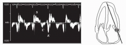
FIGURE 67.1 Tissue Doppler imaging (TDI) for diastolic function recorded from the apical four-chamber window using a 2-mm sample volume positioned in the lateral wall 1 cm from the mitral annulus. The TDI signal is toward the transducer in systole (S) as the myocardium moves toward the apex. In diastole, the myocardial velocity is directed away from the transducer first with early diastolic filling (E′) and then with atrial contraction (A′).
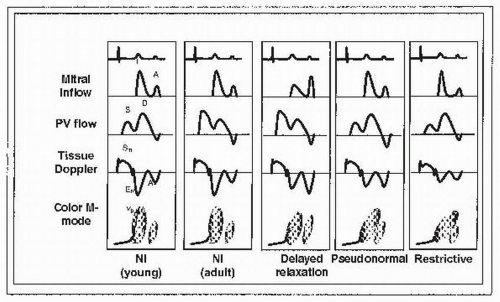
FIGURE 67.2 Diastolic function/dysfunction staging. PV, pulmonary vein; Tissue Doppler: mitral annular velocity by Tissue Doppler; Nl, normal; S, systolic; D, diastolic; Sm, systolic annular velocity; Em, early diastolic annular velocity (E′); Am, atrial annular velocity (A′); Vp, velocity of propagation; E, early mitral inflow velocity; A, atrial kick mitral inflow velocity.
D. Color M-mode (CMM).
This technique, whereby color flow Doppler is imposed on an M-mode image, permits excellent spatiotemporal distribution of velocity (color) data, although it is limited to the defined scan line. It is a valuable adjunct in the timing of cardiac events, which may not be readily appreciated by 2D and color flow imaging alone. Its primary use has been in evaluating diastolic filling pattern where the LV inflow CMM pattern typically has two appreciable waves, the first demonstrating the early passive filling wave and the second later wave resulting from atrial contraction (Fig. 67.2). The slope of the early filling wave (velocity of propagation, Vp) is primarily dependent on the rate of relaxation and is reduced with delayed relaxation. It is useful for differentiating a normal mitral inflow pattern (normal Vp) from a pseudonormal filling pattern (where impaired relaxation results in delayed flow propagation into the left ventricle, slower Vp) (Fig. 67.2 and Table 67.4).
TABLE 67.4 Diastolic Function/Dysfunction Staging
Normal young
Normal adult
Normal elderly
Delayed relaxation
Pseudonormal filling
Restrictive filling
Stage
Normal
Normal
Normal
I
II
III
E/A ratio
> 1 (often > 2)
> 1
< 1
< 1
1-2
> 2
DT (ms)
< 220
< 220
> 220
> 220
150-200
< 150
S/D ratio
< 1
≥ 1
> 1
> 1
< 1
< 1
Ar (cm/s)
< 35
< 35
< 35
< 35
> 35
> 25
Vp (cm/s)
> 55
> 55
< 55
< 55
< 45
< 45
E′ (cm/s) (E annulus)
> 10
> 8
< 8
< 8
< 8
< 8
Only gold members can continue reading. Log In or Register to continue