Systolic shortening fraction of the left ventricle

The systolic shortening fraction (SF) roughly corresponds to the pumping function of the LV, resting on the following hypothesis: the shortening of the minor axis of the LV is a reflection of the overall systolic function. In practice, this is a simple parameter to calculate. It is well correlated with the angiographic ejection fraction and is used almost systematically (Fig. 9.1). The SF is derived from the M-mode measurement of the diameters of the LV at end-diastole (EDD) and in end-systole (ESD):

Figure 9.1 Measurement of the shortening fraction (SF) and the ejection fraction (EF) of the left ventricle (LV) using M-mode. (a) The method is feasible and reliable in the case of homogeneous regional wall motion (SF = 38%; EF = 68%). (b) Measurement of the SF is not possible, because the method is invalid when there is paradoxical septal motion. AO, aorta; IVS, interventricular septum; LA, left atrium; RV, right ventricle.

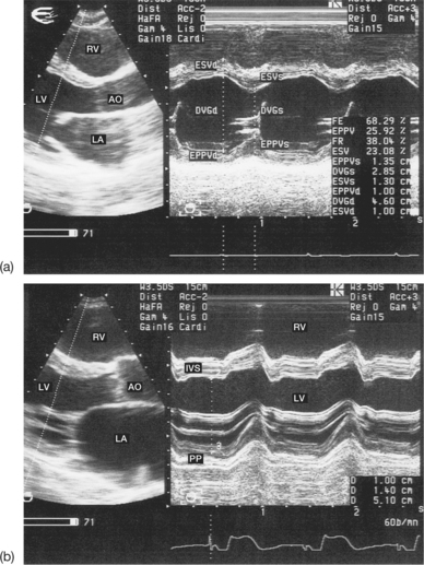
The normal value of the SF is 36 ± 6%. This parameter is, however, not ideal, because it is derived from a measurement made at only one level of the ventricle. In fact, the SF explores only the basal part of the LV and does not take into account the movement of the other ventricular segments. Thus it is possible to evaluate the overall systolic function of the LV only if its wall motion is homogeneous. The pitfalls of using the SF calculation are summarized in Box 9.2 (see also Fig. 9.1). Moreover, the interpretation of the SF values obtained is sometimes delicate. The SF depends not only on the intrinsic contractility of the LV, but also on the load conditions. Thus, an acute increase in the preload and/or a reduction in the afterload (hypotension, mitral regurgitation, etc.) leads to an increase in the SF. Conversely, an acute decrease in the preload and/or an acute increase in the afterload (e.g. tension pulse) reduces the SF.

Left ventricular ejection fraction

The ejection fraction (EF) is calculated using the end-diastolic volume (EDV) and end-systolic volume (ESV) of the LV as follows:

The normal value of the EF is 63 ± 6%.

The ventricular volumes may be calculated in one of two ways:

In practice, software integrated into the ultrasound machine allows automatic calculation of the EF according to the volumetric method selected. The EF best expresses the pumping function of the LV. It is nonetheless subject to the same errors as the evaluation of ventricular volumes (Box 9.3). In fact, the cube formula, which is based on the assimilation of the LV into a rotational ellipsoid, the major axis of which is double the minor axis, often overestimates the volumes in the case of left ventricular dilatation. When the LV is dilated, the ratio of the major axis to the minor axis decreases and is no longer equal to 2. The Teicholz formula brings a correction factor to the cube formula for the dilated or spherical LV. Whichever formula is used, the calculation is only reliable if the overall contraction of the LV is homogeneous. Obviously, the ventricular diameter as measured obliquely in M-mode, and therefore overestimated, leads inevitably to an overestimation of volume. These numerous restrictions have led to the increasingly frequent use of 2D echocardiography in daily practice to determine the ventricular volumes. Several geometric models have been proposed, on which the calculation of the volumes have been based (monoplanar or biplanar ellipsoid, disc methods, hemi-ellipse/cylinder methods, etc.). Using these different models, the estimation of the volumes is extrapolated on the basis of the ventricular surface areas measured during systole and diastole using planimetry, and of the ventricular dimensions, over one or more 2D cross-sections, according to the model applied (Fig. 9.2).

Figure 9.2 Calculation of the left ventricular (LV) ejection fraction (EF) using the ventricular volumes measured in the 2D mode according to the ‘ellipsoid monoplane’ model: (a) 2D apical image of the four chambers frozen in end-diastole and in end-systole; (b) LV systolic dysfunction (EF = 32%).

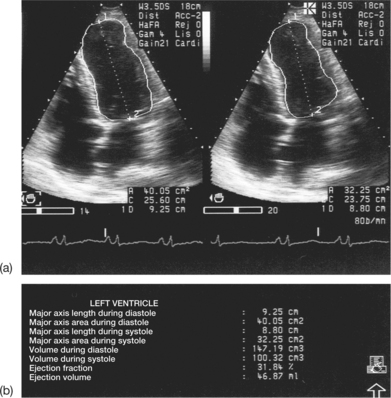
The quantification of ventricular volumes using 2D echocardiography is more precise than that done using M-mode. The 2D modality is particularly useful and advantageous in cases of deformation of the LV (e.g. aneurysm). It is also valuable in cases of regional wall motion abnormalities; this is often the case in ischaemic cardiopathy. The modality is sufficiently reproducible and reliable when used by a trained operator. However, the 2D method is not exempt from criticism and there are pitfalls in its current use that must be clearly understood (see Box 9.3).

The routine use of echocardiography shows the difficulty of optimal visualization of the endocardial contours of the LV. This is why it is so important to adjust and use the ultrasound machine correctly, and to select the most echogenic projection, and therefore the most appropriate method deriving from it. Taking an average of at least three measurements is also vital. It is also necessary to exercise prudence in the interpretation of the results, in order to avoid making an arbitrary judgement.

In fact, the left ventricular EF is highly sensitive to variations in the afterload. It is therefore necessary to interpret this parameter in the light of possible modifications in the afterload conditions (increased, as in aortic stenosis or arterial hypertension, or reduced, as in mitral regurgitation).

Technological advances in ultrasound imaging (harmonic imaging; colour kinesis, based on the automatic detection of the contours of the endocardium; myocardial contrast echocardiography) have made possible considerable improvements in the definition of the endocardial contours during systole and diastole, and consequently in the calculation of ventricular volumes in the 2D mode. In parallel, the reproducibility of the examination has been strengthened as a result of these new techniques. Three-dimensional echocardiography also gives access to the measurement of the left ventricular volumes and EF.

Cardiac output

Cardiac Doppler makes it possible to calculate the cardiac output at the level of the four cardiac valves. The calculation of the aortic output (left ventricular outflow) is the simplest and most commonly used method in current practice. The aortic output (Q_AO) may be considered as a reflection of the systolic performance of the LV. It is calculated by using echo Doppler at the subaortic level, and then multiplying the subaortic velocity–time integral (VTI) by the surface area of the outflow chamber of the LV (S) and the heart rate (HR):

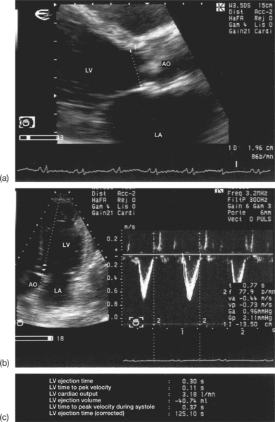
To calculate the left ventricular outflow tract area, it is sufficient to measure the subaortic diameter (D) using 2D echocardiography and the parasternal, long-axis view (Fig. 9.3):

Figure 9.3 Calculation of the cardiaic output using the echo Doppler mode. (a) Measurement of the subaortic diameter in the longitudinal, parasternal cross-section, in zoom (D = 1.96 cm). (b) Planimetry of the subaortic flow recorded using pulsed Doppler in the apical cross-section (velocity–time integral (VTI) = 13.5 cm, heart rate = 78 beats/min). (c) Aortic output: Q_AO = 3.14(D/2)² ˘ VTI ˘ HR = 3.14(1.96)² ˘ 13.5 ˘ 78 = 3.18 l/min. AO, aorta; LA, left atrium; LV, left ventricle.

In a healthy subject, the normal value of the aortic output is in the range 4–7 l/min. The Q_AO is generally corrected using the body surface area in order to determine the cardiac index. The cardiac index is considered pathological if its value is < 2.5 l/min/m².

The pitfalls of evaluating the aortic output using the echo Doppler modality are summarized in Box 9.4. They are linked in particular to:

In fact, the calculation of Q_AO in echo Doppler is based on the following assumptions:

Therefore, for the calculation of the output to be reliable, the subaortic flows should be laminar and flat. This is by no means the case when there is a rim or septal kinking. In the case of a turbulent flow with a parabolic velocity profile (higher velocity at the centre of the orifice) the calculation of the aortic output by this method should be abandoned, rather than be used to calculate a false value.

Poor alignment with the aortic flow leads to underestimation of the subaortic velocity (VTI), and therefore of the aortic output. Thus it is necessary to increase the number of projections explored by varying the site of the Doppler region of interest below the aortic orifice. It is important to note that the subaortic VTI also varies according to the heart rate (Fig. 9.4). Thus, for a given aortic surface area and a given heart rate, the VTI increases as the heart rate decreases, and vice versa.

Figure 9.4 Influence of continuous arrhythmia due to atrial fibrillation on the mitral and aortic flow: (a) disappearance of the A wave of the mitral flow; (b) variability in the velocity–time integral of the aortic flow. LA, left atrium; LV, left ventricle.

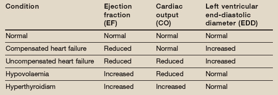
It is important to consider the basic measurements (VTI, D, HR) in order to determine the LV stroke voume precisely, reliably and reproducibly. It must be emphasized that all the measurements used to calculate the output (VTI, D, HR) are interdependent, and that an error in any one of them will produce an incorrect result. Therefore, even the smallest of errors (2 mm) in the measurement of the subaortic diameter leads to significant variations in the calculated result; hence the importance of the quality of the 2D image. Finally, the interpretation of Doppler measurements of the aortic output is also complex. The multiple determinants of the cardiac output must be taken into account. Thus, the cardiac output is not an isolated value and should be compared with other clinical (blood pressure, thyroid function, etc.), haemodynamic (venous pressure, capillary pressure, etc.) and echocardiographic (ejection fraction, left ventricular dimensions, associated valvular regurgitation, etc.) data (Table 9.1). Cardiac failure at high cardiac output may point to hypothyroidism, anaemia or an arteriovenous fistula.

Table 9.1 Some examples of haemodynamic profiles in Doppler echocardiography

As for the measurement of the output at the level of the mitral and tricuspid orifices, the measurement of the aortic output runs into major technical difficulties (elliptical shape of the orifices, continuous variation in the valve surface area during diastole, non-flat velocity profile), rendering this complex measurement less reliable and more difficult to achieve in current practice.

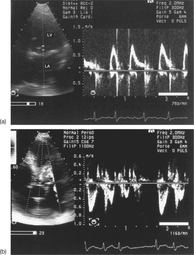
Recording and interpretation of diastolic Doppler parameters

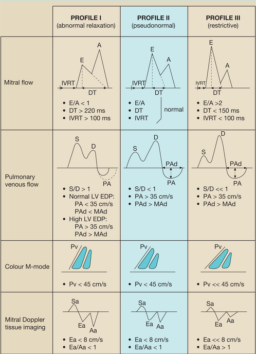
Detailed analysis of the Doppler parameters discussed below makes it possible to classify patients into three haemodynamic profiles corresponding to stages of increasing severity of the diastolic dysfunction of the LV (Table 9.2):

Table 9.2 Table 9.2 Characteristics of the three diastolic dysfunction profiles of the left ventricle (LV)

Stay updated, free articles. Join our Telegram channel

Join