 Figure 7-1 A) Normal pressure waveform. B) Pressure underdamping caused by an air bubble in the tubing. This produces high frequency oscillations that result in the peak pressures appearing higher. |
Table 7-1 Common Sources of Error in Hemodynamic Measurements | |||||||||||||||||||||||
|---|---|---|---|---|---|---|---|---|---|---|---|---|---|---|---|---|---|---|---|---|---|---|---|
|
Obtain vascular accesses, typically with an 8-Fr. sheath, allowing passage of the 7-Fr. PA (Swan-Ganz) catheter. Typically, if the pulmonary artery (PA) catheter is guided solely by pressure tracings to advance it to wedge position, the right internal jugular vein and the left subclavian vein provide the most direct anatomic routes to the pulmonary artery that matches the natural curve of the catheter.
Inflate the balloon at the tip of the catheter under water to ensure no air leak.
Make sure that all lumens of the PA catheter are flushed.
Zero the pressure transducer at the level of the mid-right atrium.
Connect the PA catheter’s distal port to the pressure transducer. Make sure that there are no bubbles in the tubing or the catheter.
Advance the catheter 20 cm through the sheath prior to balloon inflation to ensure the catheter tip clears the sheath. Do not advance if any resistance is met.
Beware of arrhythmias especially after the catheter crosses the tricuspid valve, primarily premature ventricular contractions (PVCs), and non-sustained ventricular tachycardia (NSVT). In the setting of underlying LBBB, the catheter may induce complete heart block. In the setting of myocardial infarction, the catheter may induce ventricular fibrillation.
Monitor pressures as the catheter is being advanced through the right atrium (RA), right ventricle (RV), and PA to wedge position. Be careful not to overwedge.
Do not pull back the catheter with the balloon inflated. Damage to valves, either pulmonary or tricuspid may result.
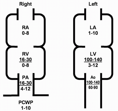 Figure 7-2 Normal hemodynamic pressure measurements in various cardiac chambers. RA, mean right atrial pressure; RV, right ventricular pressure; PA, pulmonary artery pressure; PCW, pulmonary capillary wedge pressure; LA, mean left atrial pressure; LV, left ventricular pressure. |
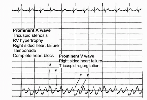 Figure 7-3 Normal RA pressures. Right atrial pressure is the same as central venous pressure and is equal to right ventricular diastolic pressure. “a” wave, right atrial systole; “x” descent, right atrial relaxation; “v” wave, right atrial filling during ventricular systole; “y”-descent, right atrial emptying. Usually, the “a” wave is higher than the “v” wave in normal patients. Giant “a” waves are seen in right-sided heart failure with a stiff right ventricle. Cannon “a” waves are seen in complete heart block when the right atrium contracts against a closed tricuspid valve. (Note: The distance between horizontal lines is 4 mm Hg, and the time between vertical lines is 1 second.) (From Topol EJ, Califf RM, et al. Textbook of Cardiovascular Medicine, 3rd Edition. Philadelphia: Lippincott Williams & Wilkins, 2006.) |
 Figure 7-4 Normal RV pressures. Right ventricular systolic pressures are elevated with right-sided heart failure, pulmonary valve stenosis, and pulmonary hypertension. Right ventricular diastolic pressures are elevated with cardiac tamponade and increased right ventricular stiffness. (Note that the distance between horizontal lines is 4 mm Hg and the time between vertical lines is 1 second.) (From Topol EJ, Califf RM, et al. Textbook of Cardiovascular Medicine, 3rd Edition. Philadelphia: Lippincott Williams & Wilkins, 2006.) |
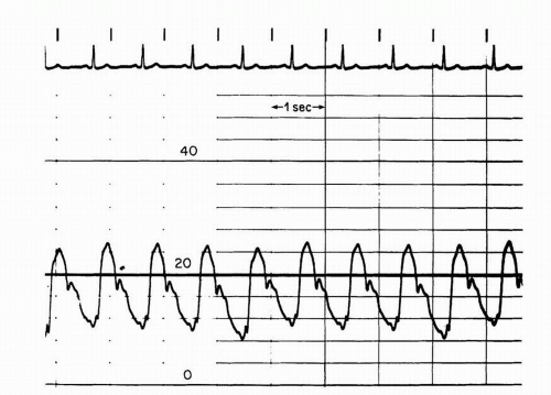 Figure 7-5 PA pressures. Pulmonary artery pressures are elevated with left-sided heart failure, lung disease, and pulmonary vascular disease. In pulmonary vascular disease, the pulmonary artery diastolic pressure can be significantly higher than the pulmonary capillary wedge pressure. This finding is most commonly found in primary pulmonary hypertension, chronic pulmonary embolism, and Eisenmenger syndrome with intracardiac shunts. (Note: The distance between horizontal lines is 4 mm Hg, and the time between vertical lines is 1 second.) (From Willard JE, Lange RA, Hillis LD. Cardiac catheterization. In: Kloner RA, ed. The guide to cardiology, 3rd. Ed. New York: Le Jacq Communications, 1995:145-164.) |
 Figure 7-6 Pulmonary capillary wedge pressures. “a” wave, left atrial systole; “v” wave, left atrial filling during ventricular systole. (Note: The distance between horizontal lines is 4 mm Hg, and the time between vertical lines is 1 second.) (Adapted from Willard JE, Lange RA, Hillis LD. Cardiac catheterization. In: Kloner RA, ed. The guide to cardiology, 3rd. Ed. New York: Le Jacq Communications, 1995:145-164.) |
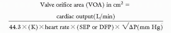
Aortic Valve Orifice Areas | |
Normal aortic orifice area | 3-4 cm2 |
Mild stenosis | >1.5 cm2 |
Moderate stenosis | 1.0-1.5 cm2 |
Severe stenosis | <1.0 cm2 |
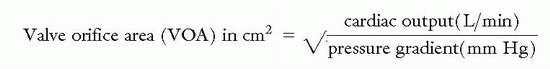
ventricle and the ascending aorta (Figure 7-7). This method allows the calculation of the mean gradient by direct measurement from both recordings. The easiest way to accomplish this is to use a dual-lumen pigtail catheter, which permits simultaneous measurement of pressures in the LV and ascending aorta.
 Figure 7-7 Simultaneous pressure tracings of left ventricle and ascending aorta, demonstrating the significant gradient across the aortic valve. (From Willard JE, Lange RA, Hillis LD. Cardiac catheterization. In: Kloner RA, ed. The guide to cardiology, 3rd. Ed. New York: Le Jacq Communications, 1995:145-164.) |
maximum left ventricular pressure (Figure 7-8). Each of these peaks occurs at different points in time, however, and this measurement is only an estimate of the mean gradient. In addition, in patients with severe aortic stenosis, the catheter itself may take up a significant fraction of the orifice area, resulting in worsened stenosis and increased gradients.
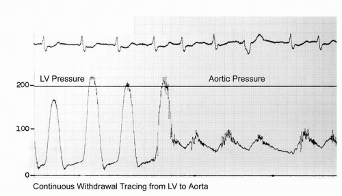 Figure 7-8 Pressure tracing of the pullback across the aortic valve. |

Stay updated, free articles. Join our Telegram channel

Full access? Get Clinical Tree


