David M. Mirvis, Ary L. Goldberger
Electrocardiography
The technology and the clinical usefulness of the electrocardiogram (ECG) have continuously advanced over the past two centuries. Early demonstrations of the heart’s electrical activity during the last half of the 19th century were closely followed by direct recordings of cardiac potentials by Waller in 1887. Invention of the string galvanometer by Einthoven in 1901 provided a direct method for registering electrical activity of the heart in humans. By 1910, the ECG had emerged from the research laboratory into the clinic and soon became the most commonly used cardiac diagnostic test.
Recent advances have extended the importance of the ECG. It is a vital test for determining the presence and severity of acute myocardial ischemia, localizing sites of origin and pathways of tachyarrhythmias, assessing therapeutic options for patients with heart failure, and identifying and evaluating patients with genetic diseases who are prone to arrhythmias. Although other techniques have evolved to assess cardiac structure, the ECG remains the basic method to assess the heart’s electrical activity. Achievements in physiology and technology have expanded the information about the heart’s electrical activity that can be derived from the ECG and will extend these clinical applications.
This chapter reviews the physiologic bases for ECG patterns in health and in disease, outlines the criteria for the most common ECG diagnoses in adults, describes critical aspects of its clinical application, and suggests future opportunities for the practice of electrocardiography.
Fundamental Principles
The ECG is the final outcome of a complex series of physiologic and technologic processes. First, transmembrane ionic currents are generated by ion fluxes across cell membranes and between adjacent cells. These currents are synchronized by cardiac activation and recovery sequences to generate a cardiac electrical field in and around the heart that varies with time during the cardiac cycle. This electrical field passes through numerous other structures, including the lungs, blood, and skeletal muscle, that perturb the cardiac electrical field.
The currents reaching the skin are then detected by electrodes placed in specific locations on the extremities and torso that are configured to produce leads, representing the difference in potentials sensed by pairs of electrodes or electrode combinations. The outputs of these leads are amplified, filtered, and displayed, using a variety of devices, to produce an ECG recording. In computerized systems, these signals are digitized, stored, and processed by pattern recognition software. Diagnostic criteria are then applied, either manually or with the aid of a computer, to produce a preliminary interpretation.
Genesis of Cardiac Electrical Fields
Ionic Currents and Cardiac Electrical Field Generation During Activation.
Transmembrane ionic currents (see Chapter 33) are ultimately responsible for the potentials that are recorded as an ECG. The process of generating the cardiac electrical field during activation is illustrated in Figure 12-1. A single cardiac fiber, 20 mm in length, is activated by a stimulus applied to its leftmost margin (Fig. 12-1A). Transmembrane potentials (Vm) are recorded as the difference between intracellular and extracellular potentials (Φi and Φe, respectively).
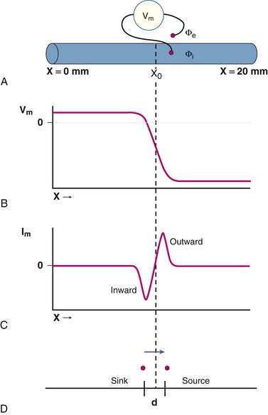
Figure 12-1B plots Vm along the length of the fiber at the instant (t0) at which activation has reached the point designated as X0. As each site is activated, it undergoes depolarization, and the polarity of the transmembrane potential converts from negative to positive, as represented in the typical cardiac action potential. Thus sites to the left of the point X0 that have already undergone excitation have positive transmembrane potentials (i.e., the inside of the cell is positive relative to the outside of the cell), whereas those to the right of X0 that remain in a resting state have negative transmembrane potentials. Near the site undergoing activation (site X0), the potentials reverse polarity over a short distance.
Figure 12-1C displays the direction and magnitude of transmembrane currents (Im) along the fiber at the instant (t0) at which excitation has reached site X0. Cardiac electrophysiologic currents are considered to be the movement of positive charge. Current flow is inwardly directed in fiber regions that have just undergone activation (i.e., to the left of point X0) and outwardly directed in neighboring zones still at rest (i.e., to the right of X0). Sites of outward current flow are current sources and those with inward current flow are current sinks. As depicted in the figure, current flow is most intense in each direction near the site of activation, X0.
Because the border between inwardly and outwardly directed currents is relatively sharp, these currents may be visualized as if they were limited to the sites of maximal current flow, as depicted in Figure 12-1D, and separated by a small distance, d, which usually is 1.0 mm or less. As activation proceeds along the fiber, the source-sink pair moves to the right, that is, in the direction of activation, at the speed of propagation in the fiber.
Cardiac Wave Fronts.
This example from one cardiac fiber can be generalized to the more realistic case in which multiple adjacent fibers are activated in synchrony to produce an activation wave front. The electrical fields generated by a wave front can be represented by a single vector (or dipole) with a strength and orientation equal to the vector sum of all of the fields generated by each of the simultaneously active fibers.
Such an activation wave front generates an electrical field that is characterized by positive potentials ahead of the front and negative potentials behind it. This relationship between the direction of movement of an activation wave front and the polarity of potentials is critical in electrocardiography: An electrode senses positive potentials when an activation front is moving toward it and negative potentials when the activation front is moving away from it.
The potential recorded by an electrode at any site within this field is directly proportional to the average rate of change of intracellular potential as determined by action potential shapes and the size of the wave front; inversely proportional to the square of the distance from the activation front to the recording site; and directly proportional to the cosine of the angle between the axis of the direction of activation and a line drawn from that axis to the recording site.
Cardiac Electrical Field Generation During Ventricular Recovery.
The cardiac electrical field during recovery (phases 1 through 3 of the action potential—see Chapter 33) is generated by forces analogous to those described during activation. However, recovery differs in several important ways from activation, including the orientation, strength, and propagation speed of the wave front.
First, intercellular potential differences and, hence, the directions of current flow during recovery are the opposite of those described for activation. As a cell undergoes recovery, its intracellular potential becomes progressively more negative. For two adjacent cells, the intracellular potential of the cell whose recovery has progressed further is more negative than that of the adjacent, less recovered cell. Intracellular currents then flow from the less recovered toward the more recovered cell—that is, recovery wave fronts will have an orientation opposite that of activation wave fronts.
The strength of the recovery front also differs from that of the activation front. As noted earlier, the strength of a wave front is proportional to the rate of change in transmembrane potential. Rates of change in potential during the recovery phases of the action potential are considerably slower than during activation, so that the strength of the recovery fronts at any one instant during recovery is less than during activation.
A third difference between activation and recovery is the rate of movement of the activation and recovery wave fronts. Activation is rapid (as short as 1 millisecond in duration) and occurs over only a small distance along the fiber. Recovery, by contrast, lasts 100 milliseconds or longer and occurs simultaneously over extensive portions of the heart.
These features result in characteristic electrocardiographic differences between activation and recovery patterns. All other factors being equal (an assumption that often is not true, as described later), ECG waveforms generated during recovery of a linear fiber with uniform recovery properties would be of opposite polarity, lower amplitude, and longer duration in comparison with those generated by activation. As described further on, these features are explicitly demonstrated in the clinical ECG.
Role of Transmission Factors.
These activation and recovery fields exist within a complex three-dimensional physical environment, referred to as the volume conductor, which modifies the cardiac electrical field. The contents of the volume conductor are called transmission factors to emphasize their effects on transmission of the cardiac electrical field throughout the body.
They may be grouped into four broad categories—cellular factors, cardiac factors, extracardiac factors, and physical factors. Cellular factors determine the intensity of current fluxes that result from local transmembrane potential gradients. Lower concentrations of the sodium ion, for example, reduce the intensity of current flow and reduce extracellular potentials.
Cardiac factors affect the relationship of one cardiac cell to another. The two major factors are (1) the more rapid propagation of activation along the length of a fiber than across its width, resulting in greater current flow in that direction, and (2) the presence of connective tissue between cardiac fibers that disrupts efficient electrical coupling of adjacent fibers. Recording electrodes oriented along the long axis of a cardiac fiber register higher potentials than for electrodes oriented perpendicular to the long axis. Waveforms recorded from fibers with little or no intervening connective tissue are narrow in width and smooth in contour, whereas those recorded from tissues with abnormal fibrosis are prolonged, with prominent notching.
Extracardiac factors encompass all the tissues and structures that lie between the activation region and the body surface, including the ventricular walls, intracardiac blood, lungs, skeletal muscle, subcutaneous fat, and skin. These tissues alter the cardiac field because of differences in the electrical resistivity of adjacent tissues to produce electrical inhomogeneities within the torso. For example, intracardiac blood has much lower resistivity (162 Ω cm) than the lungs (2150 Ω cm). Differences in torso inhomogeneities can have significant effects on ECG potentials, especially when the differences are exaggerated as in obese persons.
Other transmission factors reflect basic laws of physics (i.e., physical factors). Potential magnitudes change in proportion to the square of the distance between the heart and recording electrode. A related factor is the eccentricity of the heart within the chest. The right ventricle and anteroseptal aspect of the left ventricle are closer to the anterior chest wall than are other parts of the left ventricle and atria. Therefore ECG potentials will be higher on the anterior than on the posterior chest, and waveforms projected from the anterior left ventricle to the chest wall will be greater than those generated by posterior regions.
An additional physical factor affecting the recording of cardiac signals is cancellation. When two or more wave fronts that are simultaneously active during activation (or repolarization) have different orientations, the vectorial components of the wave fronts are oriented in opposite directions. These forces cancel each other when viewed from remote electrode positions. The magnitude of this effect is substantial. During both the QRS and ST-T waves, as much as 90% of cardiac activity is obscured by cancellation.
As a result of all of these factors, body surface potentials have an amplitude of only 1% of the amplitude of transmembrane potentials, are smoothed in detail so that surface potentials have only a general spatial relationship to the underlying cardiac events, preferentially reflect electrical activity in some cardiac regions over others, and manifest only limited amounts of total cardiac electrical activity.
Recording Electrodes and Leads
Potentials generated by the cardiac electrical generator and modified by transmission factors are sensed by electrodes placed on the torso that are configured to form various types of leads.1
Electrode Characteristics.
ECG potentials are affected by the properties of the dermal and epidermal layers of the skin, the electrode itself, and the mechanical contact between the electrode and skin. The net effect is equivalent to a complex electrical circuit that includes resistances, capacitances, and voltages produced by these different components and the interfaces between them. In clinical practice, using an electrolytic paste and cleaning the skin with a mild abrasive can improve electrode-skin contact and reduce the artifacts produced by these factors.
Electrocardiographic Lead Systems.
The standard clinical ECG is recorded from electrodes placed on each of the four extremities and six placed on the chest. These electrodes are connected to form leads that record the potential difference between two electrodes (or, as described later, electrode sets). One electrode is designated as the positive input. The potential at the other, or negative, electrode (or electrode set) is subtracted from the potential at the positive electrode to yield the bipolar potential. The actual potential at either electrode is not known, and only the difference between them is recorded. The American Heart Association (AHA) and other cardiology societies recommend that all ECG leads be referred to as bipolar leads, because they register the potential difference between two electrodes.*
In some cases, as described later, multiple electrodes are electrically connected together to represent the negative member of the bipolar pair. This electrode network or compound electrode is referred to as a reference electrode. The lead then records the potential difference between a single electrode serving as the positive input, the exploring electrode, and the potential in the reference electrode.
The clinical ECG is performed using 12 such leads: three standard limb leads (leads I, II, and III), six precordial leads (leads V1 through V6), and three augmented limb leads (leads aVR, aVL, and aVF). Specifics of electrode placement and definitions of the positive and negative inputs for each lead are presented in Table 12-1.
TABLE 12-1
Location of Electrodes and Lead Connections for the Standard 12-Lead Electrocardiogram and Additional Leads
| LEAD TYPE | POSITIVE INPUT | NEGATIVE INPUT |
| Standard Limb Leads* | ||
| I | Left arm | Right arm |
| II | Left leg | Right arm |
| III | Left leg | Left arm |
| Augmented Limb Leads | ||
| aVR | Right arm | Left arm plus left leg |
| aVL | Left arm | Right arm plus left leg |
| aVF | Left leg | Left arm plus right arm |
| Precordial Leads† | ||
| V1 | Right sternal margin, fourth intercostal space | Wilson central terminal |
| V2 | Left sternal margin, fourth intercostal space | Wilson central terminal |
| V3 | Midway between V2 and V4 | Wilson central terminal |
| V4 | Left midclavicular line, 5th intercostal space | Wilson central terminal |
| V5 | Left anterior axillary line at the same horizontal plane as for the V4 electrode‡ | Wilson central terminal |
| V6 | Left midaxillary line at the same horizontal plane as for the V4 electrode | Wilson central terminal |
| V7 | Posterior axillary line at the same horizontal plane as for the V4 electrode | Wilson central terminal |
| V8 | Posterior scapular line at the same horizontal plane as for the V4 electrode | Wilson central terminal |
| V9 | Left border of spine at the same horizontal plane as for the V4 electrode | Wilson central terminal |
* Limb electrodes should be placed near the wrists and ankles or, at a minimum, distal to the shoulders and hips.
† The right-sided precordial leads V3R to V6R are placed in mirror image positions on the right side of the chest.
‡ If the anterior axillary line is difficult to delineate, the electrode may be placed midway between the V4 and V6 electrode positions.
Standard Limb Leads.
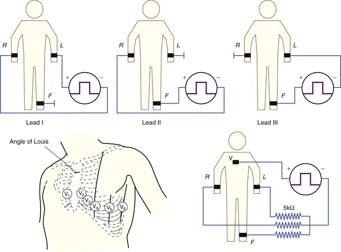
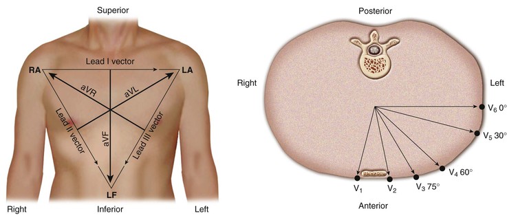
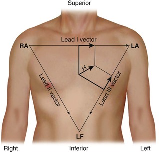
The standard limb leads record the potential differences between two limbs, as detailed in Table 12-1 and illustrated in Figure 12-2 (top). Lead I represents the potential difference between the left arm (positive electrode) and right arm (negative electrode), lead II displays the potential difference between the left leg (positive electrode) and right arm (negative electrode), and lead III represents the potential difference between the left leg (positive electrode) and left arm (negative electrode). The electrode on the right leg serves as an electronic reference that reduces noise and is not included in these lead configurations.
The electrical connections for these leads form a triangle, known as the Einthoven triangle. In it, the potential in lead II equals the sum of potentials sensed in leads I and III, as shown by this equation:

This relationship is known as Einthoven’s law or Einthoven’s equation.
Precordial Leads and the Wilson Central Terminal.
The precordial leads register the potential at each of the six designated torso sites (see Fig. 12-2, bottom, left panel) in relation to a reference potential. To accomplish this, an exploring electrode is placed on each precordial site and connected to the positive input of the recording system (see Fig. 12-2, bottom right). The negative input is the mean value of the potentials recorded at each of the three limb electrodes, referred to as the Wilson central terminal (WCT).†
The potential in each V lead can be expressed as

where

and Vi is the potential recorded in precordial lead i, Ei is the voltage sensed at the exploring electrode for lead Vi, and WCT is the potential in the composite Wilson central terminal. Thus the potential in the Wilson central terminal is the average of the potentials in the three limb leads.
The potential recorded by the Wilson central terminal remains relatively constant during the cardiac cycle, so that the output of a precordial lead is determined predominantly by time-dependent changes in the potential at the precordial site. The waveforms registered by these leads preferentially reflect potentials generated in cardiac regions near the electrode, with lesser contributions by those generated by more distant cardiac sources active at any instant during the cardiac cycle.
Precordial electrode placement in women with large breasts may be problematic. Most often, the electrodes are placed beneath the breasts, to reduce attenuation of recorded voltages and to reduce motion artifact.1
Augmented Limb Leads.
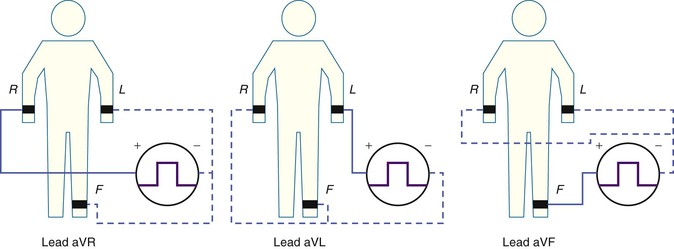
The three augmented limb leads are designated aVR, aVL, and aVF. The exploring electrode (Fig. 12-3) that forms the positive input is the right arm electrode for lead aVR, the left arm electrode for lead aVL, and the left leg electrode for aVF. The reference potential for the augmented limb leads is formed by connecting the two limb electrodes that are not used as the exploring electrode. For lead aVL, for example, the exploring electrode is on the left arm and the reference electrode is the combined output of the electrodes on the right arm and the left foot.
Thus

and
This modified reference system was designed to produce a larger-amplitude signal than if the full Wilson central terminal were used as the reference electrode. When the Wilson central terminal was used, the output was small, in part because the same electrode potential was included in both the exploring and the reference potential inputs. Eliminating this duplication results in a theoretical increase in amplitude of 50%.
The three standard limb leads and the three augmented limb leads are aligned in the frontal plane of the torso. The six precordial leads are aligned in the horizontal plane of the chest.
As described previously, individual extremity electrodes are included in more than one lead. This results in significant redundancy in the information recorded by the six frontal plane leads. The previous lead equations indicate that all six frontal plane leads can be computed from recordings at any two limb leads. Indeed, ECG machines commonly record potentials from only two of the three limb electrodes and then compute the potentials in all six frontal plane leads. By contrast, each of the six precordial electrodes provides unique information without such redundancy.1
The 12 leads are commonly divided into subgroups corresponding to the cardiac regions to which they are thought to be most sensitive. Various definitions of these groupings have been offered in the literature. For example, anterior lead groups have been defined as including V2 through V4 or only V2 and V3, and leads I and aVL have been described as being lateral or anterobasal. These designations are nonspecific, and the recommendation of expert committees has been not to use them in ECG interpretation, except in the case of localizing myocardial infarction.2
Other Lead Systems.
Other lead systems have been developed to detect diagnostically important information not recorded by the standard 12-lead ECG and to increase the efficiency of recording, transmitting, and storing an ECG. Such systems include expanded lead sets that include leads in addition to the standard 12 leads and lead sets based on electrodes in nonstandard locations.
Expanded lead systems include the recording of additional right precordial leads to assess right ventricular abnormalities, such as right ventricular infarction in patients with evidence of inferior infarction,2 and left posterior leads (see Table 12-1) to detect acute posterolateral infarctions.
Other expanded systems include electrode arrays of 80 or more electrodes deployed on the anterior and posterior torso to display body surface potentials as body surface isopotential maps. These maps portray cardiac potentials over broader areas of the torso than those included in routine electrocardiography. This additional information may have diagnostic importance improving the accuracy of, for example, detecting ST-segment elevation acute myocardial infarction.3
Other lead sets are based on electrode configurations that differ from those in the standard ECG. These have sought to minimize movement artifacts during exercise and long-term monitoring by placing limb electrodes on the torso rather than on the limbs, and to reduce the number of electrodes to decrease the time and mechanical complexity of a full recording during emergency situations and long term monitoring.4 Specific examples are discussed in other chapters.
Although these lead sets do meet specific needs in certain clinical situations, the waveforms they produce are significantly different from those recorded from the standard ECG sites. Placing limb electrodes on the torso, for example, alters the characteristics of the limb lead electrodes as well reference electrodes used for the precordial and augmented limb leads and thereby impact all twelve leads. The result is significantly altered frontal plane QRS and ST-T wave patterns that change the mean QRS axis with impact on the diagnostic criteria for, for example, ventricular hypertrophy and myocardial infarction.5 Thus, although these modified lead sets offer advantages under specific clinical conditions, they should not be used to record a diagnostic ECG.
Other lead systems that have had clinical usefulness include those designed to record a vectorcardiogram (VCG). The VCG depicts the orientation and strength of a single cardiac dipole or vector that best represents overall cardiac activity at each instant during the cardiac cycle. Lead systems for recording the VCG record the three orthogonal or mutually perpendicular components of the dipole moment—the horizontal (x), frontal (y), and sagittal or anteroposterior (z) axes. Clinical use of the VCG has waned in recent years, but as described later, vectorial principles remain important for understanding the origins of ECG waveforms.
Lead Vectors and Heart Vectors.
A lead can be represented as a vector referred to as the lead vector. For simple two-electrode leads, such as leads I, II, and III, the lead vectors are directed from the negative electrode toward the positive one (Fig. 12-4). For the augmented limb and precordial leads, the origin of the lead vectors lies at the midpoint of the axis connecting the electrodes that comprise the compound electrode. That is, for lead aVL, the vector points from the midpoint of the axis connecting the right arm and left leg electrodes toward the left arm (Fig. 12-4, left). For each precordial lead, the lead vector points from the center of the triangle formed by the three standard limb leads to the precordial electrode site (Fig. 12-4, right).
As described earlier, instantaneous cardiac activity also can be approximated as a single vector (the heart vector) representing the vector sum of the various active wave fronts. Its location, orientation, and intensity vary from instant to instant as cardiac activation proceeds.
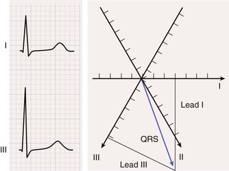
The amplitude of the potentials sensed in a lead equals the length of the projection of the heart vector on the lead vector, multiplied by the length of the lead vector:

where L and H are the length of the lead and heart vectors, respectively, and θ is the angle between the two vectors, as illustrated in Figure 12-5. Thus, if the projection of the heart vector on the lead vector points toward the positive pole of the lead axis, the lead will record a positive potential. If the projection is directed away from the positive pole of the lead axis, the potential will be negative. If the projection is perpendicular to the lead axis, the lead will record zero potential.
Hexaxial Reference Frame and Electrical Axis.
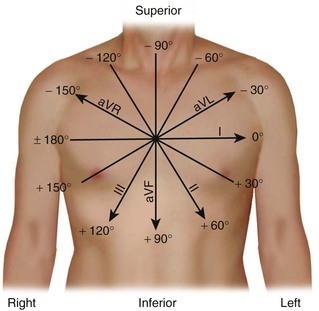
The lead axes of the six frontal plane leads can be superimposed to produce the hexaxial reference system. As depicted in Figure 12-6, the six lead axes divide the frontal plane into 12 segments, each subtending 30 degrees.
These concepts allow calculation of the mean electrical axis of the heart. The orientation of the mean electrical axis represents the direction of activation in an “average” cardiac fiber. This direction is determined by the properties of the cardiac conduction system and activation properties of the myocardium. Differences in the relation of cardiac to torso anatomy contribute relatively little to shifts in the axis. As described further on, this measurement is an important part of diagnostic criteria for chamber enlargement and conduction system defects.
The process for computing the mean electrical axis during ventricular activation in the frontal plane is illustrated in Figure 12-7. First, the mean force during activation is represented by the area under the QRS waveform, measured as millivolt-milliseconds. Areas above the baseline are assigned a positive polarity and those below the baseline have a negative polarity. The overall area equals the sum of the positive and the negative areas.
Second, the area in each lead (typically, two are chosen) is represented as a vector oriented along the appropriate lead axis in the hexaxial reference system (see Fig. 12-6), and the mean electrical axis equals the resultant or vector sum of the two vectors. An axis directed toward the positive end of the lead axis of lead I—that is, oriented directly away from the right arm and toward the left arm—is designated as an axis of 0 degrees. Axes oriented in a clockwise direction from this zero level are assigned positive values, and those oriented in a counterclockwise direction are assigned negative values.
The mean electrical axis during ventricular activation in the horizontal plane can be computed in an analogous manner by using the areas under and lead axes of the six precordial leads (see Fig. 12-4, right). A horizontal plane axis located along the lead axis of lead V6 is assigned a value of 0 degrees, and those directed more anteriorly have positive values.
This process can be applied to compute the mean electrical axis for other phases of cardiac activity. Thus the mean force during atrial activation is represented by the areas under the P wave, and the mean force during ventricular recovery is represented by the areas under the ST-T wave.
Electrocardiographic Processing and Display Systems
ECG recording using computerized systems involves six steps: (1) signal acquisition; (2) data transformation; (3) waveform recognition and feature extraction; (4) diagnostic classification; (5) data compression and storage; and (6) display of the final ECG.1
Signal Acquisition.
Signal acquisition steps include amplifying the recorded signals, converting the analog signals into digital form, and filtering the signals to reduce noise. The standard amplifier gain for routine electrocardiography is 1000. Lower (e.g., 500 or half-standard) or higher (e.g., 2000 or double-standard) gains may be used to compensate for unusually large or small signals, respectively.
Analog signals are converted to a digital form at rates of 1000/second (1000 Hz) to as high as 15,000 Hz. Too low a sampling rate will miss brief signals such as notches in QRS complexes or pacemaker spikes and will result in altered waveform morphologies. Too fast a sampling rate may introduce artifacts, including high-frequency noise, and will generate excessive amounts of data necessitating extensive digital storage capacity.
ECG potentials are then filtered to reduce unwanted, distorting signals. Low-pass filters reduce the distortions caused by high-frequency interference from, for example, muscle tremor and external electrical devices; high-pass filters reduce the effects of body motion or respiration. For routine electrocardiography, the standards set by professional groups require an overall bandwidth of 0.05 to 150 Hz for adults.1 Narrower filter settings, such as 1 to 30 Hz, as commonly used in rhythm monitoring, will reduce baseline wander related to motion and respiration but may result in significant distortion of both the QRS complex (including width, amplitude, and Q wave patterns) and the ST-T wave.1
Stay updated, free articles. Join our Telegram channel

Full access? Get Clinical Tree


