Scott D. Solomon, Justina Wu, Linda Gillam, Bernard Bulwer
Echocardiography
Echocardiography remains the most commonly used and comprehensive cardiac imaging modality and is generally considered the first test of choice for assessing cardiac structure and function in most clinical situations. When compared with other imaging methods, echocardiography can be performed quickly, with minimal patient inconvenience or discomfort, and provides immediate clinically relevant information at relatively low cost. Echocardiography provides detailed data on cardiac structure, including the size and shape of cardiac chambers, as well as the morphology and function of cardiac valves. Furthermore, the real-time nature of echocardiography makes it uniquely suited to noninvasive assessment of systolic and diastolic function and intracardiac hemodynamics. In most echocardiography laboratories, standard transthoracic echocardiography (TTE) is complemented by transesophageal echocardiography (TEE), which offers improved resolution because of closer proximity of the transducer to cardiac structures, and by stress echocardiography, which is routinely used to assess myocardial ischemia and valvular function with exercise. Technical advancements in echocardiography over the past several decades have led to progressively improved diagnostic capabilities, including major advances in three-dimensional echocardiography, miniaturization of equipment leading to handheld echocardiography units, and contrast echocardiography for better cavity visualization and assessment of myocardial perfusion.
Because two-dimensional echocardiography is not a tomographic technique like cardiac computed tomography (CT) or cardiac magnetic resonance (CMR) (see Chapters 17 and 18), acquisition of ultrasound images is dependent on an operator—either a sonographer or a physician—applying an ultrasound transducer to a patient’s chest. Both acquisition and interpretation of echocardiograms require substantial training and skill. Thus echocardiography is best described as an “examination” rather than a “test.” Although cardiologists receive this training routinely, a growing number of noncardiologists, including emergency physicians, anesthesiologists, intensivists, and others, are increasingly using echocardiography in their practice. The advent of small, handheld ultrasound devices, which complement the physical examination, will further open this field to a wide array of practitioners who may not currently practice echocardiography. Knowledge of its basic principles, uses, and limitations is becoming essential for all physicians who care for patients with cardiovascular problems.
Principles of Ultrasound and Instrumentation
Principles of Image Generation
Echocardiography is based on the standard principles of ultrasound imaging in which high-frequency sound waves in the 1- to 10-MHz range are emitted from piezoelectric crystals housed in a transducer, traverse through internal body structures, interact with tissues, reflect back to the transducer, and are then processed by microcomputers to generate an image. An understanding of the physical principles that underlie echocardiography is essential to understanding its usefulness and limitations.1
Ultrasound machines calculate the time required for sound waves to reflect from structures and return to the transducer, thereby determining the depth of reflecting structures. This information is used to generate scan lines that comprise data on both location (depth of reflection) and amplitude (intensity of reflection). Early ultrasound equipment projected a single “beam” of ultrasound, which resulted in a single scan line that could be “painted” across a moving paper or screen, with depth being depicted on the vertical axis and time on the horizontal axis. This method, known as M-mode (for “motion”) echocardiography (Fig. 14-1, right panel), has largely been replaced by two-dimensional imaging (Fig. 14-1, left panel), although it is still used routinely and considered ideal for making linear measurements and for assessments that require high temporal resolution.
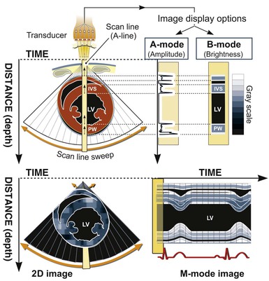
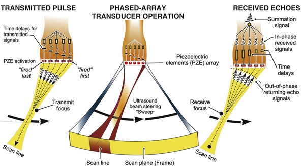
Two-dimensional imaging uses electronically steered, phased-array transducers with multiple (currently up to 512) emitting and receiving elements embedded in the transducer (Fig. 14-2). These devices emit pulses of ultrasound in an ordered sequence and sequentially listen for returning echoes, referred to as the pulse-echo principle. The sequence occurs repeatedly to generate moving images. The rate at which these pulses are emitted, termed the pulse repetition frequency (PRF), is limited by the finite speed of ultrasound in tissues (≈1540 meters/sec) and the depth of the tissues being interrogated because time is required for the ultrasound pulse to return to the transducer. Nevertheless, improvements in processing speed have allowed “frame” rates to reach speeds higher than 100 per second. For most imaging applications, frame rate, a determinant of temporal resolution, can be increased by narrowing the scan sector, imaging at shallower depths, and reducing scan line density. Three-dimensional echocardiography extends the phased-array concept to a planar waffle-like grid or matrix-array transducer and allows both simultaneous multiplanar two-dimensional imaging and true volumetric three-dimensional imaging and rendering (see the section Three-Dimensional Echocardiography).
Principles of Doppler Imaging
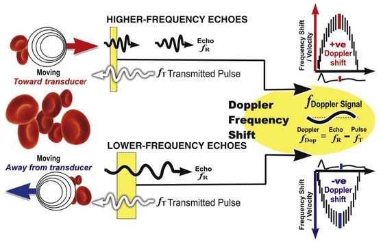
In addition to generating images of cardiac structures, ultrasound can be used to interrogate the velocity of blood flow through the heart and to quantify movement of the cardiac chambers. These techniques are based on the Doppler principle, which states that the frequency of any waveform emitted from a moving object will be perceived as higher than or lower than the actual frequency, depending on whether the object is moving toward or away from the observer. Ultrasound that is emitted at a particular frequency and then reflected from moving red blood cells will return to the transducer at a slightly different frequency than that at which it was emitted: either higher if the flow is toward the transducer or lower if the flow is away from the transducer (Fig. 14-4). This difference between the frequency emitted and that received, termed the Doppler frequency shift, is dependent on the speed of ultrasound through the medium and the velocity of blood flow and is summarized by the Doppler equation
where fd is the Doppler shift frequency, ft is the transmitted ultrasound frequency, V is the velocity of blood flow, c is the speed of ultrasound in the tissue, and θ represents the angle of flow relative to the ultrasound beam (angle of insonation).
Pulsed-Wave and Continuous-Wave Doppler
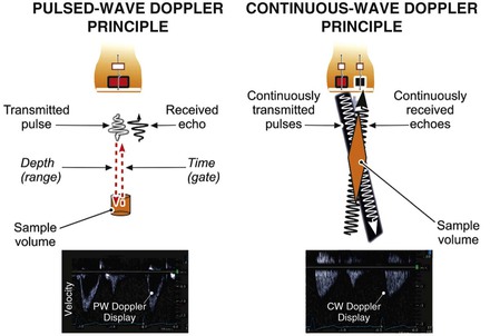
The two principal types of Doppler imaging are pulsed-wave (PW) and continuous-wave (CW) Doppler (Fig. 14-5). In PW Doppler (Fig. 14-5, left panel), discrete pulses of ultrasound reflect off moving structures (i.e., red blood cells moving through the heart) and return to the transducer. By gating (i.e., defining a specific time window in which to listen to the reflected signal), this technique can be used to assess the velocity of blood flow at a particular depth within the heart. When an operator places a cursor on the two-dimensional ultrasound image at a particular location, the equipment will assess the velocity at that particular location. Because these pulses take time to reflect and return to the transducer, they cannot be transmitted too frequently or the equipment will fail to discern whether a given pulse—or a later pulse—has returned and the velocity information obtained at that depth will be ambiguous. The PRF is essentially the sampling rate; the higher the blood flow velocity, the higher the frequency of the Doppler shift and hence the higher the sampling rate needed to accurately sample that shift. From a practical standpoint, these physical principles determine the upper limit of velocities that can be interrogated accurately with PW Doppler. The Nyquist limit refers to the maximum velocity that can be accurately quantified within a given sample volume and is directly related to the PRF, which in turn is inversely related to the distance from the sample volume to the transducer (Fig. e14-1 ).
).
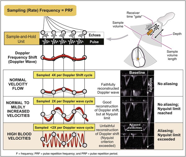
 , this difference, the Doppler frequency shift, is directly related to the velocity of the flowbeing assessed. The sampling rate is essentially the PRF. If this rate is too low, the waveform being sampled (in this case the Doppler shift waveform) cannot be approximated by the system, and the waveform will be sampled ambiguously. PW Doppler can accurately sample and reconstruct lower blood velocities (from the Doppler shift) with no ambiguity (aliasing)
 With CW Doppler (see Fig. 14-5, right panel) a dedicated piezoelectric element continuously emits ultrasound and a separate element simultaneously continuously receives the returning signals. Because the ultrasound tone is continuous rather than pulsed, depth localization cannot be ascertained from the signal received. However, unlike the situation with PW Doppler, no limit is imposed on the velocities discernible with this technique. Thus PW Doppler is primarily used to assess flow with relatively low velocity (typically <1.5 meters/sec) present at a specific depth location, whereas CW Doppler is used to assess higher velocities (typically >1.5 meters/sec) but without such depth specificity.
Color Flow Doppler
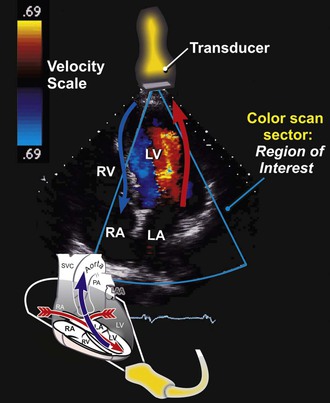
Color flow Doppler is a PW Doppler–based technique in which the velocities in a region of interest are encoded with colors that represent both mean velocities and directionality of the flow superimposed on a two-dimensional image with a color map (Fig. 14-6). By convention, flow that is moving away from the transducer is encoded in blue, and flow that is moving toward the transducer is encoded in red. Because color flow Doppler is a form of PW Doppler, it is subject to aliasing. High velocities and turbulent flow, when a wide range of velocities exist, appear as a multicolored mosaic pattern (usually green and yellow). In some systems the variance in the velocities relative to the mean is color-coded in superimposed shades of green. Color flow Doppler allows direct real-time visualization of the movement of blood in the heart and is particularly useful in identifying blood flow acceleration and turbulence. Hence color flow Doppler is exceptionally adept at delineating regurgitant lesions, which tend to be relatively high-velocity flow and turbulent, and discrete stenoses, in which blood flow accelerates.
Blood Flow Profiles and Doppler Signals
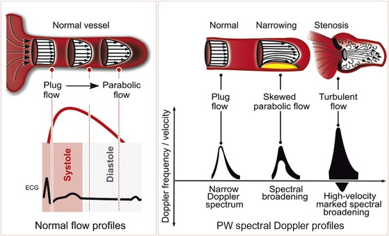
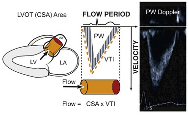
Blood flow through the heart and major blood vessels can be laminar or turbulent. Laminar, or streamlined, flow occurs when the direction and velocity of flow throughout a region are uniform (Fig. 14-7). Blood flow through a normal heart and great vessels is predominantly laminar, even across valves. The spectral Doppler flow signal observed when interrogating laminar flow is characterized by a “hollowed-out” waveform, indicative of the narrow range or spectrum of flow velocities present within the sample. In a Doppler assessment of the left ventricular (LV) outflow tract (LVOT), for example, the Doppler profile represents the velocity of blood flow throughout systole. If this flow is primarily laminar, blood flow velocities within the sample region will be relatively uniform at each instant during the cardiac cycle. If the flow becomes turbulent, with blood moving at different velocities or in multiple directions, the spectrum of velocities will be wider.
As illustrated by the Doppler equation (see earlier), the velocity of blood flow determined from the Doppler shift will change as the angle of insonation changes. Practically, this means that if the vector of flow is not directly in line with the ultrasound beam, the velocities calculated by the Doppler shift will be underestimated. This problem can be corrected by applying an angle adjustment at the machine level, although the further the angle of flow deviates from the angle of the beam, the greater the likelihood for error in the calculation, and in general it is best to avoid Doppler assessments that are substantially off-angle.
Doppler Echocardiography in Practice
Doppler echocardiography is used primarily to assess blood flow velocity in the heart and blood vessels. Within the heart the velocity of blood flow is itself dependent on the pressure gradient between cardiac chambers, with higher gradients resulting in higher velocities. Knowledge of the velocity of blood flow between two chambers, for example, can be used to infer the pressure gradient between them. This relationship can be described by the Bernoulli equation, which estimates the pressure gradient between two chambers separated by an orifice based on the velocity of flow through the orifice:
where P1 and P2 are the pressures proximal and distal to the orifice and V1 and V2 are the velocities proximal and distal to the orifice. In practice, a simplified form of the Bernoulli equation that ignores flow acceleration and viscous friction can be used:
The equation can be even further simplified because velocities proximal to an orifice or stenosis are generally quite low in comparison to those distal to the orifice and can usually be ignored, which leaves
For example, the blood flow velocity of tricuspid regurgitation (TR) can be used to calculate the pressure gradient between the right ventricle and the right atrium, which when added to an estimate of right atrial (RA) pressure, provides an estimate of pulmonary artery systolic pressure. Similarly, the highest blood flow velocity between the left ventricle and the aorta in a patient with aortic stenosis can be used to calculate the peak instantaneous pressure gradient across the aortic valve. It is important to appreciate that Doppler echocardiography measures velocity, neither pressure nor flow directly. Pressure gradients can be inferred from velocities based on the Bernoulli equation, but absolute pressure within chambers cannot be directly measured as in cardiac catheterization. Similarly, volumetric flow cannot be measured directly, although there are Doppler-based methods that permit estimation of flow relatively precisely.
Assessment of Flow and Continuity Equation
Even though Doppler methods are used to assess blood flow velocities, the magnitude of flow can be inferred by multiplying the velocity-time integral (VTI; i.e., integrated velocity throughout the cardiac cycle) by the cross-sectional area (CSA) of the region being interrogated (Fig. 14-8). For example, stroke volume (SV) can be estimated by interrogating the LVOT region with PW Doppler and multiplying the VTI by the CSA (which is calculated by measuring the diameter):

The continuity principle, which is based on conservation of mass and states that flow in one region of the heart should be equivalent to flow in another region (assuming no intervening shunt), can be used to determine an unknown CSA, such as that of a stenotic valve. The CSA of a stenotic valve can be difficult to measure directly (i.e., by planimetry); by estimating the flow proximal to the valve and the VTI through the valve, valve area can be determined. Even though velocities through stenotic valves can be too high to assess with PW Doppler, CW Doppler can be used, assuming that the highest attained velocities correspond to the narrowest region along the Doppler path being interrogated. Because the continuity principle states that flow through the LVOT must equal flow through the aortic valve (AV),

solving for AreaAV yields an estimate of the desired valve area. The accuracy of this estimate depends on the accuracy of the known CSA measurement and optimal positioning of the PW Doppler cursor.
The Standard Adult Transthoracic Echocardiographic Examination
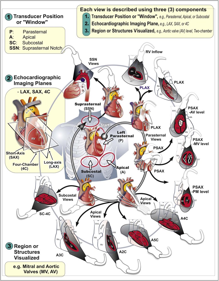
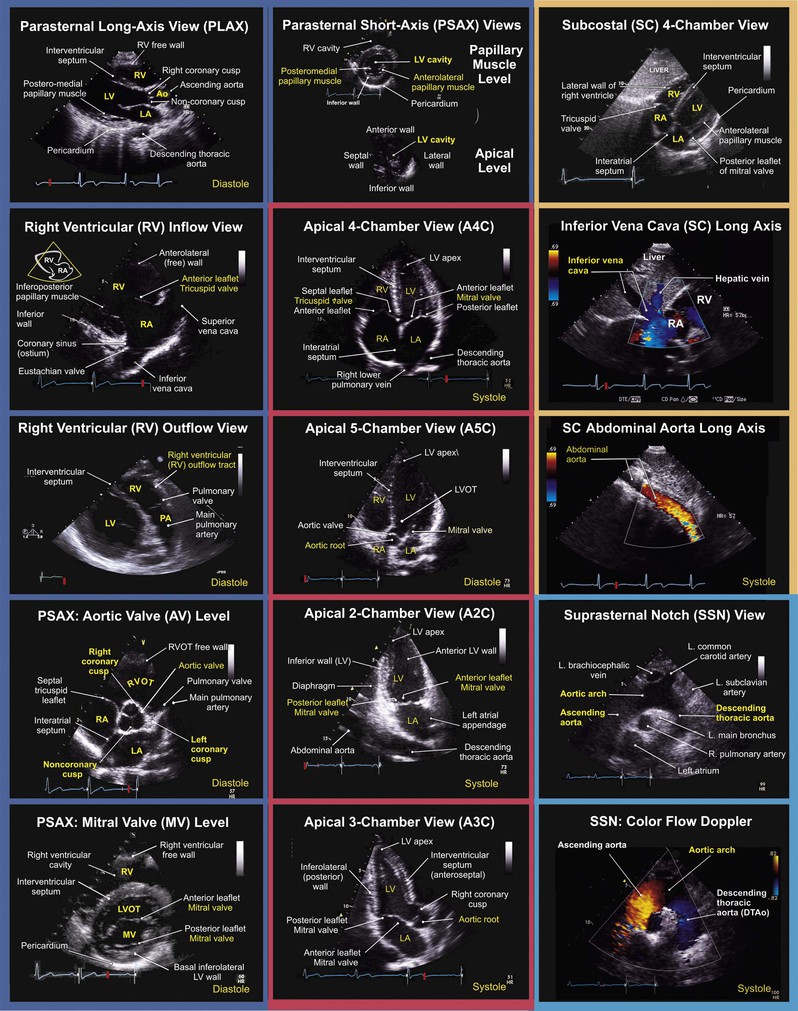
The standard adult TTE examination consists of a combination of two-dimensional, M-mode, and Doppler imaging. The recommended comprehensive examination protocol involves optimal image acquisition of echocardiographic views, each of which is described in terms of three principal components: (1) the standard transducer position or “windows,” (2) the orthogonal echocardiographic imaging planes, and (3) the anatomic region of interest (Figs. 14-9 and 14-10). At each transducer position the operator optimally acquires two-dimensional images with color flow Doppler, spectral Doppler, or M-mode images as indicated.
M-Mode Echocardiography
M-mode echocardiography (see Fig. 14-1) provides greater temporal resolution than does standard two-dimensional imaging and remains the method of choice for certain linear measurements, particularly those that are collinear with the ultrasound beam, such as measurement of septal and posterior wall thickness and LV chamber dimensions on parasternal views. Because M-mode echocardiography is essentially a one-dimensional imaging technique, this method has several important limitations that should be recognized, especially when M-mode–derived data are used to determine information about cardiac size and shape. In particular, M-mode–based estimates of LV volume, mass, and function can be inaccurate in patients with LV geometries that deviate substantially from normal, such as following myocardial infarction (MI). M-mode can also be combined with color flow Doppler (color M-mode) to provide accurate timing-related information about flow and has been used for assessment of diastolic function (see later).
Imaging Artifacts
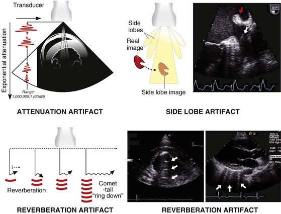
Ultrasound imaging artifacts are ubiquitous in echocardiography and in large measure are products of the physical principles of ultrasound. Artifacts can include the appearance of structures that do not exist or can be the result of structures that do exist, such as ribs obscuring proper visualization of existing structures. Although imaging artifacts can result from faulty ultrasound equipment, interference from other electronic equipment, or improper ultrasound machine settings, most artifacts are due to physical interactions between ultrasound and tissue. Several types of artifacts are common (Fig. 14-11), including (1) attenuation artifacts, which result in “shadowing” typically caused by ribs or bony structures; (2) reverberation artifacts, which are caused by internal reflections; (3) side lobe artifacts, which occur when structures reflected from “side lobes” of the ultrasound beam are erroneously mapped onto the image; and (4) rib “dropout” artifacts, in which cardiac structures are obscured because of the marked ultrasound attenuation caused by the bony rib cage. One type of artifact, the comet-tail artifact, can be useful diagnostically to detect interstitial fluid in the lungs.
Assessment of Cardiac Structure and Function
The primary goal of the echocardiographic examination remains assessment of cardiac structure and function. Each chamber and valve can be assessed qualitatively and quantitatively by experienced operators to define any alterations in cardiac size and geometry by using comprehensive measurements. Established normal values are shown in Tables 14-1 through 14-5. Measurements of cardiac structures are typically made in various locations throughout the heart, and linear, area, or volumetric measures can be obtained. These methods are often complementary to one another; for example, although volumetric measurements of the left ventricle (see later) are generally considered best suited to characterize LV size, many laboratories continue to record linear cavity measurements, a practice that is supported by the extensive literature correlating these measures with outcomes in numerous disease states. Moreover, linear measures can be subject to less variability than area- or volume-based measures and can therefore be more reliable when assessing changes over time.
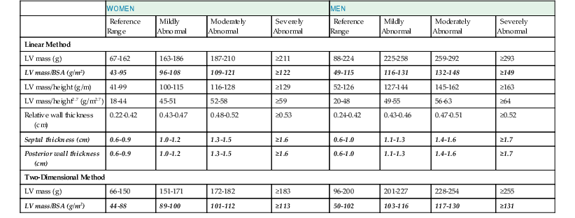
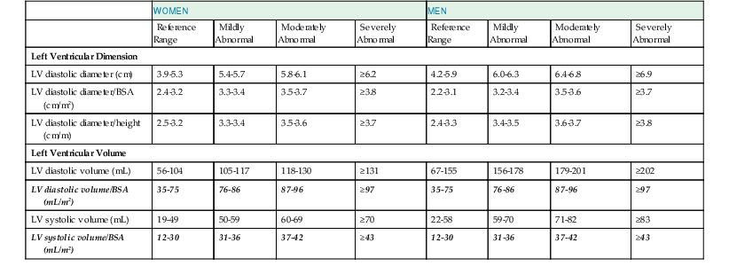
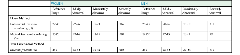
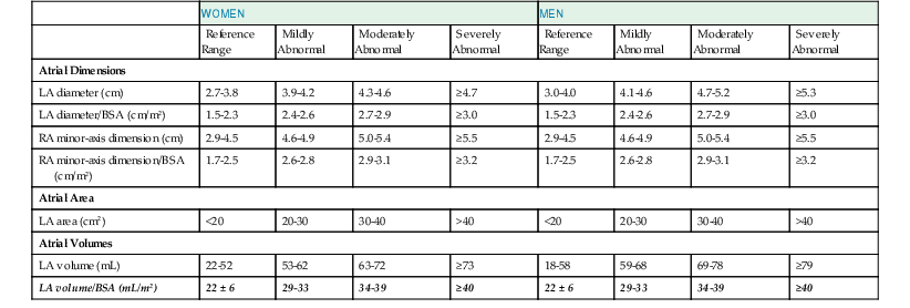
TABLE 14-5
Summary of Reference Limits for Recommended Measures of Right-Sided Heart Structure and Function
| VARIABLE | UNIT | ABNORMAL |
| Chamber Dimensions | ||
| RV basal diameter | cm | >4.2 |
| RV midcavity diameter | cm | >3.5 |
| RV longitudinal diameter | cm | >8.6 |
| RV end-diastolic area | cm2 | >25 |
| RV end-systolic area | cm2 | >14 |
| RV end-diastolic volume indexed | mL/m2 | >80 |
| RV end-systolic volume indexed | mL/m2 | >46 |
| Three-dimensional RV end-diastolic volume indexed | mL/m2 | >89 |
| Three-dimensional RV end-systolic volume indexed | mL/m2 | >45 |
| RV subcostal wall thickness | cm | >0.5 |
| RVOT PSAX distal diameter | cm | >2.7 |
| RVOT PLAX proximal diameter | cm | >3.5 |
| RA major dimension | cm | >5.3 |
| RA minor dimension | cm | >4.4 |
| RA end-systolic area | cm2 | >18 |
| Systolic Function | ||
| TAPSE | cm | <1.6 |
| Pulsed Doppler peak velocity at the annulus | cm/s | <10 |
| Pulsed Doppler MPI | — | >0.40 |
| Tissue Doppler MPI | — | >0.55 |
| FAC | % | <35 |
| Diastolic Function | ||
| E/A ratio | — | <0.8 or >2.1 |
| E/E′ ratio | — | >6 |
| Deceleration time | msec | <120 |
MPI = myocardial performance index; PLAX = parasternal long axis; PSAX, parasternal short axis.
Left Ventricular Structure: Size and Mass
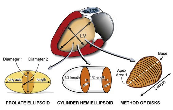
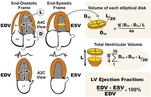
LV volumes can be estimated from one of several formulas that use either linear or two-dimensional measurements to calculate a volume based on the assumption that the left ventricle approximates a prolate ellipsoid (Fig. 14-12). These approaches are limited when ventricular geometry deviates substantially from normal, as is the case in patients with MI, in whom the ventricle can be substantially distorted. The single-plane or biplane Simpson method of discs is an approach that does not rely on such rigid geometric assumptions and has been demonstrated to be the most accurate method (Fig. 14-13). This method requires manually identifying the endocardial border in the apical four- and/or two-chamber views with computerized assistance to measure the diameter of equally distributed slices along the ventricle. A CSA is calculated from this diameter by assuming a circle if the single-plane method is used or an ellipse if two orthogonal planes are used. Even though the Simpson method is usually more accurate than other methods of assessing ventricular volumes, precise identification of the endocardial border can be challenging when image quality is reduced. Moreover, foreshortening of the ventricle in one of the apical views, which can occur simply by minor changes in the transducer angle, can dramatically reduce the measured volume and adversely affect volumetric estimations. Three-dimensional echocardiography has the potential to reduce some of the inherent limitations of two-dimensional imaging (see Three-Dimensional Imaging, later).
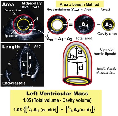
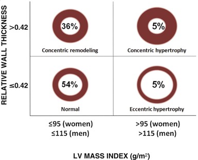
LV mass may be calculated by using one of several formulas that take into account both wall thickness and chamber size2 (Fig. 14-14; see Table 14-1). These formulas have been validated in geometrically normal ventricles, but their accuracy is markedly reduced in the setting of altered ventricular geometry, such as following MI. LV hypertrophy is defined by the overall LV mass. In general, if LV diameter is not decreased, wall thickness of 12 mm or greater is usually indicative of LV hypertrophy (see Table 14-1). Both myocardial and valvular diseases can result in remodeling of the left ventricle and hence abnormal ventricular geometry. Categorization of ventricular geometry is based on relative wall thickness and the LV mass index (Fig. e14-2 ). The specific pattern of ventricular remodeling has been related to prognosis in a variety of diseases.2
Left Ventricular Systolic Function
Echocardiography offers several methods for assessment of systolic function. The LV ejection fraction (LVEF), calculated as the difference between end-diastolic volume and end-systolic volume divided by end-diastolic volume, remains the most commonly used method for assessing systolic function. It is one of the best-studied measures in cardiovascular medicine and has proved useful in diagnosis and risk stratification in a variety of cardiovascular diseases. Although accurate assessment of LVEF requires calculation from ventricular volumes, many echocardiography laboratories estimate LVEF visually. Even though calculation of LVEF from volumes is preferred, the accuracy of this estimation is affected by image quality, endocardial border definition, ventricular geometry, and representative orthogonal imaging planes. When one or more of the aforementioned factors are suboptimal, visual estimation by experienced echocardiographers can be more accurate and sufficient for most clinical scenarios.
Other approaches are commonly used in addition to LVEF to assess systolic function. SV can be determined by subtracting end-systolic volume from end-diastolic volume (calculated as described earlier) or through Doppler methods. Multiplying the VTI in the LVOT, assessed with PW Doppler on the apical four-chamber view, by the cross-sectional diameter at the same location (measured on the parasternal long-axis view) yields SV (see Fig. 14-8), which can be multiplied by the heart rate to obtain cardiac output.
Several other novel methods have been proposed for assessment of systolic function. The myocardial performance index, also known as the Tei index, is defined as the sum of isovolumic relaxation time and isovolumic contraction time divided by ejection time, and this method takes into account both systolic and diastolic performance, with a lower index being associated with better function.2 In adults, values of the LV index lower than 0.40 and RV index lower than 0.30 are considered normal. This measure has been related to outcomes in a variety of conditions, including heart failure and following MI. Doppler tissue imaging (DTI) can be used to assess myocardial contraction velocity, or S′, although this technique has proved more useful for assessment of diastolic function (see Doppler Tissue Imaging later).
Myocardial Strain Imaging
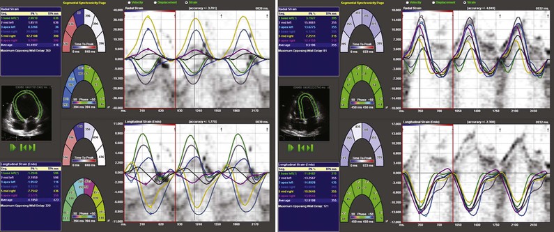
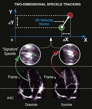
Myocardial deformation, or strain, imaging is a relatively novel yet promising method for assessment of cardiac function. Strain refers to the percent deformation between two regions and reflects shortening in myocardial muscle.3 Myocardial strain can be assessed by Doppler methods in which myocardial tissue velocities in multiple regions are integrated to obtain change in distance. Doppler-based assessments of myocardial strain are relatively noisy and require dedicated acquisition during scanning, thus limiting their usefulness. In addition, Doppler-derived strain information is angle dependent. In contrast, strain imaging based on speckle-tracking techniques has proved to be much more robust and reliable, although it has poorer temporal resolution than Doppler-based techniques do, thus limiting its use at high heart rates. Nevertheless, two-dimensional methods have virtually replaced Doppler-based strain assessments for most applications. These techniques take advantage of the coherent speckle within the myocardial tissue signature to determine regions that are contracting versus those that are moving passively (Figs. 14-15 and e14-3 ). Myocardial strain measures have been validated with sonomicrometry,4 and strain can be estimated in the longitudinal, circumferential, and radial directions by using the appropriate imaging plane (see Fig. 14-15). Speckle methods can also be used to assess ventricular twist and torsion, or the wringing motion of the heart during contraction and relaxation.
Stay updated, free articles. Join our Telegram channel

Full access? Get Clinical Tree


