Echocardiography: Basic Principles and Imaging
Haleh C. Heydarian
Thomas R. Kimball
Despite increasing use of complimentary imaging modalities such as computed tomography and magnetic resonance imaging (1,2), echocardiography remains the principal diagnostic modality in the field of pediatric cardiology (3). The echocardiography laboratory is often the patient’s last “diagnostic stop” before surgical or catheter intervention, which necessitates the most complete anatomic and physiologic description of the cardiovascular system possible and requires exquisite detail in performing the echocardiographic evaluation. In addition, pediatric imagers face two important challenges today: (a) To define the complementary roles of echocardiography and the other imaging technologies in the evaluation of congenital heart disease patients (4) and (b) to oversee the expanding utilization of echocardiography among cardiology colleagues and noncardiology healthcare providers—utilization precipitated by poorer auscultatory skills of personnel and increased miniaturization and decreased cost of cardiac ultrasound technology (5,6).
History
In 1877, 18-year-old Pierre Curie found the basis for the field that would later be known as ultrasound by discovering the piezoelectric effect in which mechanical distortion of crystals produces an electric potential and vice versa. Although this was a landmark discovery, it was not until many years later, in fact not until after the 1912 sinking of the Titanic (which catalyzed efforts to create systems aiding ships in earlier detection of icebergs), that the field of ultrasound began to develop (7). Eventually, in World War II, ultrasound waves formed the basis of Sound Navigation and Ranging (SONAR) (8).
The successful use of ultrasound as a diagnostic medical technique was simultaneously pioneered in the 1940s and 1950s by four groups: (a) the Massachusetts Institute of Technology (MIT; Bolt, Ballatine, Ludwig, and Heuter), (b) the University of Illinois (Fry, Fry, and Kelly) (c) the University of Colorado (Howry and Holmes), and (d) the University of Minnesota (Wild and Reid). The MIT group developed A (amplitude)-mode ultrasound, a method of displaying the intensity of reflected waves as spikes of various heights on an oscilloscope. The Illinois group is renowned for using ultrasound to detect breast cancer. The Colorado group developed B (brightness)-mode imaging, a method of displaying the intensity of the reflected ultrasound waves as dots of various brightness along a single scan line, the progenitor to two-dimensional (2-D) ultrasound. The Minnesota group perfected pulsed ultrasound techniques that permit a single transducer to act as both a transmitter and a receiver in real time and, by incorporating a water interface in the transducer head, creating the first hand-held scanner, thus eliminating the need for patient immersion (7,8).
Applying ultrasound for cardiac diagnosis was first performed at the University of Lund, Sweden (Edler and Hertz) in 1953. A B-mode detector with continuous moving film to obtain real-time images of the heart in waveform provided the first M(motion)-mode echocardiogram (7,8). Twenty years later, M-mode echocardiography was applied to congenital heart disease by Goldberg, Allen, Sahn et al. (9,10). In the late 1970s and early 1980s, the application of 2-D echocardiography to congenital heart disease allowing complete, accurate, and detailed diagnoses was successfully completed by pioneers such as Sahn, Snider, Silverman, Williams, Stevenson, and others (11,12,13,14,15,16,17,18,19,20). In the 1990s, ultrasound technology became increasingly miniaturized so that echocardiography began to enjoy even broader use including as a bedside adjunct to the physical examination in more unique settings such as the emergency room and the intensive care unit. With the advent of the new century, echocardiographers are employing increased use of three-dimensional (3-D) echocardiography and more sophisticated tools in the evaluation of ventricular function.
Physics of 2-D Echocardiography
The piezoelectric effect, first discovered by Curie, occurs when an electric potential applied to a crystal results in mechanical distortion because of alignment of the crystal’s molecular dipoles. This, in turn, causes the crystal to resonate producing ultrasonic waves. A sound wave requires a deformable medium for its propagation because it is mechanical in nature, consisting of a series of compressions and expansions (rarefaction) of the molecules in the medium. The velocity of this sound wave depends on the type of tissue through which it is traveling (1,540 m/s in soft tissue, 330 m/s in air). The wave has characteristics that define its existence (Fig. 12.1).
The echocardiographic transducer does not emit ultrasound continuously but rather emits pulses rapidly (∼1,000 pulses/s) and quickly (∼1 ms for every pulse). Therefore, the transducer is operating as a transmitter for an extremely short time (0.1% of the time) and as a receiver for the vast majority of its operation. During a 30-minute examination, the transducer will have transmitted pulses for <2 seconds.
Eight Equations that Form the Basis of 2-D and Doppler Echocardiography
Equation 1: The Basis of Image Generation
where
%R = percent reflection of ultrasound signal
Zn = impedance in mediumn = ρncn
ρn = density of mediumn
cn = speed of sound in mediumn
As an ultrasound beam travels through the body, some of its energy will be reflected back to the transducer and some of
its energy will continue to be transmitted forward; similar to the concept of momentum, which is equal to the mass × velocity of a moving object. Consider the well-known novelty of a set of metallic balls suspended adjacent to each other as a pendulum (Fig. 12.2). When an outside ball of sufficient mass is drawn away from the stationary balls and released, it strikes the stationary balls, resulting in the outside ball on the opposite side to move away from the stationary balls. If the first outside ball were, however, the size of a pea, it would strike the stationary balls and merely bounce away from them. It does not have sufficient momentum (because of relatively small mass) to cause any perturbation in the stationary balls. It is therefore merely reflected backward.
its energy will continue to be transmitted forward; similar to the concept of momentum, which is equal to the mass × velocity of a moving object. Consider the well-known novelty of a set of metallic balls suspended adjacent to each other as a pendulum (Fig. 12.2). When an outside ball of sufficient mass is drawn away from the stationary balls and released, it strikes the stationary balls, resulting in the outside ball on the opposite side to move away from the stationary balls. If the first outside ball were, however, the size of a pea, it would strike the stationary balls and merely bounce away from them. It does not have sufficient momentum (because of relatively small mass) to cause any perturbation in the stationary balls. It is therefore merely reflected backward.
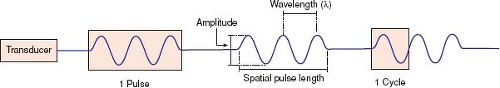 Figure 12.1 The anatomy of a wave. Sound travels with a velocity (c) dependent on the medium through which it propagates (for soft tissue, c = 1,540 m/s). The wavelength (λ) is the distance between two consecutive and equivalent parts. The frequency (υ) is the number of compressions per unit of time expressed in Hertz. The frequency and wavelength are inversely proportional to each other through the velocity of sound (υλ = c). The amplitude is the pressure difference between nadir and peak. In echocardiography, waves are emitted as pulses consisting of wave cycles. Therefore, the spatial pulse length is the distance from the beginning of a single pulse train to its end. |
Acoustic impedance is the ultrasound equivalent to momentum; tissue density replaces mass, and speed of sound replaces velocity (21). If the tissue density is the same between two media (the equivalent of a large metallic ball in the example above), the impedance between the two media is similar and ultrasound will be readily transmitted through the media interface; however, a mismatch in the tissue density between the two media (e.g., between the left ventricular wall and its cavity) will result in reflection of ultrasound (the equivalent of a pea-sized ball in the example above).
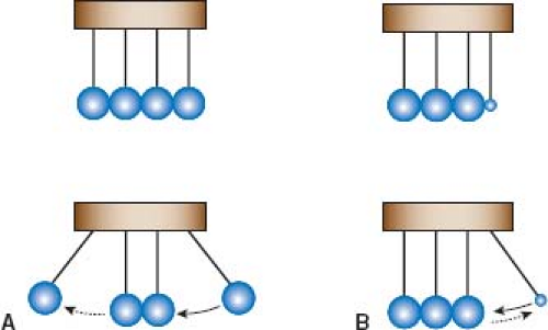 Figure 12.2 In mechanics, energy transfer is dependent on momentum. A: An outside ball equivalent in size to the stationary balls is released. It strikes the stationary balls, resulting in movement of the outside ball on the opposite side. The ball has sufficient momentum to cause effective energy transfer to the stationary balls. B: After an outside ball of smaller size is released, it strikes the stationary balls and is reflected off of them. This ball has insufficient momentum to result in energy transfer. Acoustic impedance is the ultrasound equivalent to momentum. In ultrasound, energy transfer is dependent on impedance. If the impedances between two media are similar, ultrasound will be readily transmitted. If there is a mismatch in impedance, ultrasound will be reflected. |
Equation 2: The Basis of Image Resolution (Part I)
where
SPL = spatial pulse length
λ = wavelength
n = number of cycles in a pulse of ultrasound
c = speed of sound
υ = transmission frequency
Axial resolution (resolution along the axis of the ultrasound beam) of a nonpulsed wave is proportional to its wavelength (λ) or inversely proportional to its frequency (υ) since (λ) = (c/υ). A bat feeding at twilight emits ultrasound waves at a frequency of 100 kHz, which provides excellent resolution for catching insects in air (λ = c/υ = 330 m/s ÷ 100,000 cycles/s = 3.3 mm) but provides an unacceptable resolution for cardiac anatomy if a wayward bat were to send sound waves through a patient’s chest (1,540 m/s ÷ 100,000 cycles/s = 15.4 mm). With pulsed ultrasound, the axial resolution is dependent not only on the wavelength but also the number of wave cycles in that ultrasound pulse. The best possible axial-point separation resolution is equal to 1/2 of the spatial-pulse length (Fig. 12.3). Using Equation 2, a 10-MHz transducer emitting a train of three pulsed ultrasonic waves will yield a point separation resolution of approximately 0.46 mm (3 × 154,000 cm/s ÷ 10,000,000 cycles/s). A 2.5-MHz transducer will have an approximate resolution of 1.8 mm. The poorer axial resolution of a transducer of this frequency therefore limits its usefulness in evaluating anatomy of smaller magnitude, for example, the luminal diameter of a coronary artery.
Equation 3: The Basis of Image Resolution (Part II)
where
D = depth of near field
d = diameter of transducer
υ = transmission frequency of transducer
c = speed of sound
Lateral resolution is the ability to resolve objects that are perpendicular to the beam axis and is dependent not only on wavelength (and thus transducer frequency) like axial resolution but also on the beam width. For a nonfocused transducer, the ultrasonic beam consists of a near field with narrow beam width and good lateral resolution (the Fresnel zone) and a far field where the beam width diverges rapidly limiting resolution (the Fraunhofer zone) (21). The depth of the near field (with best resolution) is extended by increasing the frequency or the footprint diameter of the transducer (Equation 3 and Fig. 12.4).
An example is afforded by imaging a newborn. For the parasternal and apical views, a small-diameter, high-frequency probe is advantageous because the cardiac structures are at a near depth
(within the Fresnel zone of the transducer) and the small footprint can be placed between the acoustically unfriendly ribs. For subcostal imaging, a larger-diameter transducer provides great advantage by extending the near field to the relatively deep depth of the cardiac structures improving their resolution.
(within the Fresnel zone of the transducer) and the small footprint can be placed between the acoustically unfriendly ribs. For subcostal imaging, a larger-diameter transducer provides great advantage by extending the near field to the relatively deep depth of the cardiac structures improving their resolution.
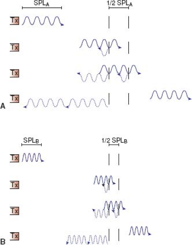 Figure 12.3 The axial resolution (resolution along the axis of the ultrasound beam) is dependent on the spatial pulse length (SPL). The shorter the SPL, the better the resolution. Resolution can be no better than 1/2 of the SPL. A: The transducer emits pulses of sound waves (solid line) with a relatively long SPL of SPLA. This train of pulses can distinguish two objects that are separated by a distance of 1/2 SPLA but no closer because the transducer would not be finished receiving the reflected wave from the proximal object before arrival of the reflected wave from the distal object. B: The transducer emits pulses of sound with a shorter SPL of SPLB. These train of pulses can distinguish two objects that are closer together but still no closer than 1/2 SPLB (reflected waves shown as dashed lines). |
Lateral resolution can be improved by focusing which causes the beam width to narrow more distally where it would otherwise begin to diverge. Focusing can be accomplished by external devices (such as mirrors or lenses) or by electronic means; however, focusing results in greater far-field divergence than with a nonfocused beam.
Equation 4: The Yin–Yang Relationship Between Resolution and Penetration
where
L = intensity attenuation loss (in decibels)
µ = intensity attenuation coefficient ∼0.8 dB/cm/MHz for soft tissue
υ = transducer frequency (in MHz)
z = distance traveled in the medium by ultrasound wave (in cm)
The energy of the ultrasound wave is decreased by tissue interactions. Attenuation describes the loss of intensity resulting from scattering (reflection at small interfaces) and absorption (energy transformation) (21). Equation 4 demonstrates that intensity loss is greatest (or penetration is poorest) not only at deeper tissue depths (z) but also when using a transducer with a higher frequency, precisely the frequency needed to enhance resolution (Equations 2 and 3). Thus, echocardiography requires a constant balancing act between optimizing resolution without sacrificing penetration and vice versa.
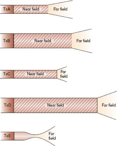 Figure 12.4 The lateral resolution (resolution perpendicular to the axis of the ultrasound beam) is dependent not only on transmission frequency but also on the beam width of the transducer. The beam is relatively narrow in the near field of the transducer. In the far field, the ultrasound beam begins to diverge and lateral resolution deteriorates. Transducer A has a relatively small diameter and, therefore, a relatively shallow near field. The diameter of transducer B is larger, thereby extending the near field. Near-field depth can be increased even when using a smaller-diameter transducer if transducer frequency is increased (transducer C). Near-field depth is optimized with transducers having relatively large diameters and emitting ultrasound of high frequency (transducer D). Lateral resolution can also be improved by focusing the transducer crystal; however, focusing has the disadvantage of the beam diverging rapidly beyond the focal zone (transducer E). |
Equation 5: The Basis of Temporal Resolution
where
F = frame rate
c = speed of sound
D = sampling depth
N = number of sampling lines per frame
n = number of focal zones used to produce one image
Motion during 2-D echocardiography is portrayed by rapid presentation of successive single-image frames, similar to viewing a motion picture film. A single-image frame is generated by successive electronic stimulation of each element in the transducer to initiate
an ultrasound pulse, which propagates down (and is received up) successive scan lines (one scan line typically extends through 1 to 3 degrees of the sector). In addition, the superimposition of a color Doppler sector on the image increases the time for a pulse to propagate down and up a scan line. The time required for the pulse to travel down one scan line to the depth of interest and back to the transducer imposes a restriction on how quickly the next element is stimulated, how rapidly a frame is acquired, and how soon the next frame can be produced. The frame rate (expressed in Hz) quantitates the speed of this process (21).
an ultrasound pulse, which propagates down (and is received up) successive scan lines (one scan line typically extends through 1 to 3 degrees of the sector). In addition, the superimposition of a color Doppler sector on the image increases the time for a pulse to propagate down and up a scan line. The time required for the pulse to travel down one scan line to the depth of interest and back to the transducer imposes a restriction on how quickly the next element is stimulated, how rapidly a frame is acquired, and how soon the next frame can be produced. The frame rate (expressed in Hz) quantitates the speed of this process (21).
Temporal resolution can be optimized by narrowing the sector size (of both the image and the color Doppler region), thereby decreasing the number of scan lines, or by decreasing the depth range (Equation 5). A practical, easy-to-remember rule of thumb to optimize frame rate is to ensure that the subject of interest fills the sector wedge completely, eliminating imaging of superfluous tissue at the lateral and inferior aspects of the sector. Since M-mode and Doppler echocardiography have better temporal resolution, these modalities may be more useful when measuring events that are occurring quickly.
Equation 6: The Doppler Equation
where
υd = the observed Doppler frequency shift
υ0 = the transmitted frequency of sound
V = blood flow velocity
θ = the intercept angle between the ultrasound beam and the direction of blood flow
c = the velocity of sound in human tissue
The Doppler principle states that the frequency of a transmitted wave is altered when the source of the wave is in motion (e.g., the siren on an ambulance racing by a pedestrian). The principle is also applicable when the source of the wave is stationary and the “receiver” of the wave is in motion. The observed change in frequency under these circumstances is termed the Doppler shift, after Christian Johann Doppler, who described this phenomenon in 1842 when studying the light waves emitted with the motion of binary stars.
A stationary surfer waiting to catch a wave encounters the same number of wave crests per minute as emitted by the source. If the surfer paddles away from the beach toward the ocean, he perceives an increase in the wave frequency because he is swimming toward the wave source. If he reverses his direction and heads to the beach (away from the source), he encounters fewer wave crests. If he moves faster in either direction, the difference between the actual and observed frequency of wave crests (the frequency shift) increases.
In medical ultrasound and echocardiography, the Doppler principle is applied using transmitted sound waves to strike moving red blood cells. Sound waves are transmitted by a stationary transducer, strike red blood cells in motion, and the returning “backscattered” sound pulses are Doppler shifted in frequency in relation to the velocity and direction in which the blood cells are moving. Doppler principles are also applied to evaluate tissue motion by Doppler tissue imaging. Doppler ultrasound is used primarily to assess velocity of moving structures, whether it be the velocity of blood flow through the heart and vasculature or the velocity of the ventricular myocardium. It is therefore appropriate to rearrange the Doppler equation to solve for velocity:
As the speed of sound (c) and the transmitted frequency (υ0) are constant, and the frequency shift (υd) can be accurately measured; the main source of potential error in Doppler estimation of velocity arises from the intercept angle, θ, between the sound beam and the direction of blood/tissue motion. Consider the surfer analogy above. If the surfer were moving toward the ocean (toward the wave source) at an oblique angle, then the “frequency shift” (i.e., the difference between the actual and observed frequency of wave crests) would be less than if he were heading directly into the wave source. The observed velocity is the velocity vector parallel to the insonation beam. The true velocity of his movement would not be known unless we were to account for his oblique travel pattern relative to the wave source. This can be determined exactly by dividing the frequency shift by the cosine of θ (the intercept angle between the wave source and his direction of travel). If the true velocity vector is aligned with the ultrasound beam (i.e., θ = 0), then cos θ is 1 and the observed velocity is the true velocity. However, if the true velocity vector and insonation beam are not aligned, the observed velocity will be smaller than the true velocity, unless angle correction is performed. For intercept angles <20 degrees, cos θ is small, and is not felt to result is significant underestimation of the flow velocity. At greater intercept angles, correction for cos θ is needed.
Equation 7: The Basis of Aliasing
where
Vmax = the maximum measurable velocity of blood
c = the velocity of sound in tissue
fo = the transmitted frequency of sound
D = depth of interest
θ = the intercept angle between the ultrasound beam and the direction of blood flow
If the Doppler sampling rate is not adequate, the frequency of the reflected wave is sampled only intermittently, data must be inferred, and the wave is misinterpreted as having a lower frequency—a phenomenon called aliasing. The phenomenon is apparent in older Western movies when the wheel of a stagecoach is perceived as rotating backward when the stagecoach is obviously moving forward. The movie consists of a series of stop-action photographs, which when shown one after the other give the appearance of motion. If the stagecoach moves very fast, the wheel turns very fast and turns too great a revolutionary arc between successive photographs. This problem is solved when by decreasing the time between successive photographs the wheel turns a smaller arc between photographs (Fig. 12.5). Translating this analogy to Doppler echocardiography, aliasing velocity can be increased by increasing the time between cycles (i.e., the “period” of the wave). Since the period is the inverse of the wave frequency, decreasing the transducer frequency will increase the aliasing velocity (Equation 7). In addition, Equation 7 demonstrates that the maximum measurable velocity of blood can be increased by sampling at a shallower depth. Therefore, it may be advantageous to consider echocardiographic windows associated with less depth to the heart when sampling a high-velocity jet.
Equation 8: The Bernoulli Equation
where
ΔP = the pressure difference across an obstructive orifice
V1 = the flow velocity proximal to the obstruction
V2 = the flow velocity distal to the obstruction
ρ = the mass density of blood = 1,060 kg/m3
dV = change in velocity over time (dt)
ds = distance over which change in pressure occurs
R = viscous resistance in blood vessel
V = velocity of blood flow
The first term, ½ ρ (V22 − V12), represents convective acceleration through the flow orifice. This portion of the equation becomes 4 (V22 − V12) when substituting the blood density of 1,060 kg/m3 into the equation, multiplying by ½ and, multiplying by the
conversion factor of 0.0075 that converts kg/m/s2 (a pascal) to mm Hg. In addition, in most clinical conditions, the proximal flow velocity is <1 m/s, and is considered negligible. Thus, the first term can be simplified as 4V22. The second term (ρ∫dV/dt (ds)) describes energy expended to accelerate fluid at the onset of flow; clinical measurements are usually made at peak flow, thus, this term can be assumed to be 0. The third term R (V) describes energy lost overcoming viscous friction along the walls of the vessel, and is felt to be of little impact in most clinical circumstances.
conversion factor of 0.0075 that converts kg/m/s2 (a pascal) to mm Hg. In addition, in most clinical conditions, the proximal flow velocity is <1 m/s, and is considered negligible. Thus, the first term can be simplified as 4V22. The second term (ρ∫dV/dt (ds)) describes energy expended to accelerate fluid at the onset of flow; clinical measurements are usually made at peak flow, thus, this term can be assumed to be 0. The third term R (V) describes energy lost overcoming viscous friction along the walls of the vessel, and is felt to be of little impact in most clinical circumstances.
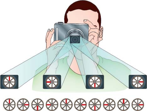 Figure 12.5 The principle of aliasing is similar to the phenomenon in old Western movies of a wheel of a stagecoach appearing to rotate backward when the stagecoach is obviously moving forward. The movie consists of a series of stop-action photographs which when placed in sequential order give the appearance of motion. If the series of photographs are captured at too low a frequency (top row) any spoke on the wheel (e.g. the highlighted, bold spike), will appear to be rotating backward (in this case, appearing to rotate 90 degrees counterclockwise each time an image is captured). It is only when the frequency of snapping photographs is high enough (bottom row), that the true forward rotation of the wheel is appreciated (in this case, rotating 90 degrees clockwise each time an image is snapped). |
It is important to understand that when the assumptions used to simplify the Bernoulli equation may not apply, the approach to estimating pressure gradients may need to be modified. A common example of such an instance is in estimation of pressure drops where the proximal velocity (V1) is greater than 1 m/s such as across an aortic coarctation, stenotic and regurgitant semilunar valves (where the regurgitant volume may result in an increase in V1), multiple obstructions in series, and in the setting of high-cardiac output. Viscous resistance may not be negligible in other circumstances where the obstruction is long and narrow (22) such as across Blalock–Thomas–Taussig shunts, or across tunnel-type obstructions, for example, tubular obstruction of the left ventricular outflow tract.
The Examination
General Considerations
Echocardiographic Windows
There are four major echocardiographic windows to the heart (Fig. 12.6): (a) parasternal, (b) apical, (c) subcostal, and (d) suprasternal notch. (A fifth window, the right parasternal window, obtained with the patient in a right lateral decubitus position, is used for obtaining an accurate Doppler gradient in patients with aortic stenosis.) The examination usually is performed in this same order, beginning with the least noxious (parasternal) window and finishing with the potentially most noxious (suprasternal notch) window. In complex cases associated with abnormal situs or cardiac position, the examination may alternatively begin with the apical or subcostal windows so that the echocardiographer can become oriented for the other views.
Parasternal and apical imaging is performed with the patient in a left lateral decubitus position. A dropout mattress may be essential for obtaining the apical view. During subcostal imaging, the patient lies supine, sometimes flexing the knees, thereby relaxing
the abdominal muscles. Suprasternal imaging is performed with a roll under the shoulders to extend the neck. When using the right parasternal view for Doppler interrogation of valvar aortic stenosis, the patient should be positioned in a right lateral decubitus position.
the abdominal muscles. Suprasternal imaging is performed with a roll under the shoulders to extend the neck. When using the right parasternal view for Doppler interrogation of valvar aortic stenosis, the patient should be positioned in a right lateral decubitus position.
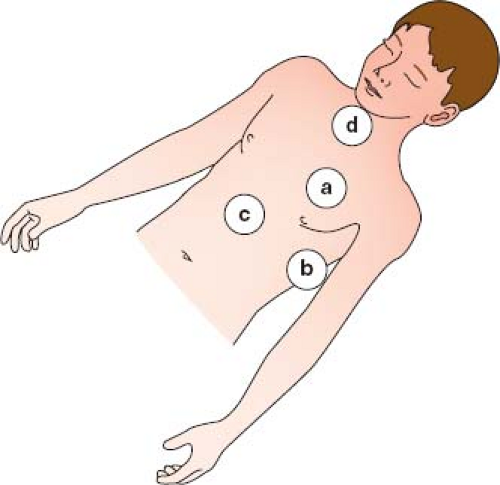 Figure 12.6 There are four main echocardiographic windows: (a) parasternal, (b) apical, (c) subcostal, and (d) suprasternal notch. The parasternal and apical windows are obtained with the patient in a left lateral decubitus position with using a dropout mattress. Subcostal images are obtained with the patient supine and sometimes with the knees flexed. Suprasternal notch images are obtained with a roll under the shoulders so that the neck is hyperextended. Additional windows include the right parasternal with the patient in a right lateral decubitus position useful for the Doppler interrogation of valvar aortic stenosis and the right apical view along the right anterior axillary line used when imaging patients with dextrocardia. |
Planes of the Heart and Technique of Sweeping: Thinking in Three Dimensions
Three-dimensional imaging is enjoying more routine use for clinical purposes. However, the challenge and essence of pediatric echocardiography continue to be acquiring all the necessary 2-D images, mentally synthesizing them into a 3-D model, and conveying this 3-D representation to others by narrative or visual tools.
The spatial location of any part of an object is defined and understood by considering it in relation to the three planes (transverse [axial], sagittal, and coronal) in which the object exists (Fig. 12.7). Each of the four standard echocardiographic windows affords the opportunity to image the heart from one or more of these three planes. From the parasternal window, the long (sagittal) and short (axial) planes are shown. From the apical and subcostal windows, the four-chamber (coronal) and two-chamber (sagittal) planes are demonstrated. Finally, from the suprasternal notch window, the sagittal and axial axes of the upper thoracic vasculature are imaged. Sweeping the transducer through the nearly parallel planes within each of the acoustic windows mimics the ability of other imaging modalities such as magnetic resonance to obtain parallel “slices” within a given plane (Figs. 12.8–12.14; Videos 12.1–12.8). With these techniques, the spatial relationships become clear, and the 3-D mental reconstruction of the heart becomes possible.
Optimizing the Doppler Examination
The robustness of Doppler echocardiography as a tool for evaluating cardiac physiology is only manifest when its practitioners exhibit precise and diligent technique. Doppler spectral envelopes need to be sharp and free of feathering. A sharp envelope is first achieved by aligning the ultrasound beam as parallel to the flow as possible. Traditionally, color Doppler is used before application of pulsed or continuous wave Doppler to determine the precise location and direction of a jet. The transducer position on the chest is then moved accordingly so that the flow is directed either exactly toward or opposite to it. The best transducer position for the Doppler examination may therefore be offset from the most ideal position for 2-D imaging. Not only the spectral display but the audio component from the Doppler signal is often helpful in determining if one is localized in the vena contracta and parallel to flow. Second, the practitioner must be careful to avoid overgaining the spectral display that can cause indistinct envelopes. Third, the spectral display of interest should fill as much of the screen as possible by shifting the baseline up or down and decreasing the Doppler scale. In this way, the envelope is made as large as possible minimizing the effect of imprecise Doppler envelope planimetry. Fourth, tracing of the Doppler envelope needs to be careful, precise, and steady.
Color Flow Doppler
The color Doppler modality interrogates flow with multiple pulsed Doppler sample volumes placed successively along multiple scan lines. For each sampling gate, the baseline frequency is compared to the received frequency. Pixels in the image are arbitrarily assigned a color (red for flow toward the transducer and blue for flow away from the transducer) and a color intensity based on the magnitude of the mean velocity. The color Doppler scale should be actively manipulated throughout the examination—using low-velocity scales when interrogating venous velocities (e.g., antegrade across/in atrioventricular valves, atrial septum, cavopulmonary shunt, and systemic and pulmonary veins) or velocities generated from lower pressure gradients (e.g., in the coronary arteries, across a large ventricular septal defect [VSD] or patent ductus arteriosus [PDA]) and high-velocity scales when interrogating arterial flows or flows
generated from high pressure gradients (e.g., atrioventricular valve regurgitation, restrictive VSD or PDA). The examiner must actively think about and anticipate expected physiology during the study so that the color scale is appropriately adjusted (Fig. 12.15). For example, in a toddler being evaluated for a suspected VSD, interrogation of the septum with a high-color Doppler scale is appropriate. However, using such a high-color scale in the investigation for a VSD in a newborn would likely miss the low velocity shunt flow since the shunt is driven by a very low pressure gradient due to the normally elevated pulmonary vascular resistance in the newborn period, that raises the right ventricular pressure. The examiner would need to interrogate the ventricular septum with a low velocity color Doppler scale in this instance. These flows then should be more carefully and precisely interrogated and quantitated with either pulsed or continuous wave Doppler. Because of the massive amount of data, a color Doppler sector should be kept as narrow as acceptable to improve accuracy and/or temporal resolution (Equation 5: The Basis of Temporal Resolution).
generated from high pressure gradients (e.g., atrioventricular valve regurgitation, restrictive VSD or PDA). The examiner must actively think about and anticipate expected physiology during the study so that the color scale is appropriately adjusted (Fig. 12.15). For example, in a toddler being evaluated for a suspected VSD, interrogation of the septum with a high-color Doppler scale is appropriate. However, using such a high-color scale in the investigation for a VSD in a newborn would likely miss the low velocity shunt flow since the shunt is driven by a very low pressure gradient due to the normally elevated pulmonary vascular resistance in the newborn period, that raises the right ventricular pressure. The examiner would need to interrogate the ventricular septum with a low velocity color Doppler scale in this instance. These flows then should be more carefully and precisely interrogated and quantitated with either pulsed or continuous wave Doppler. Because of the massive amount of data, a color Doppler sector should be kept as narrow as acceptable to improve accuracy and/or temporal resolution (Equation 5: The Basis of Temporal Resolution).
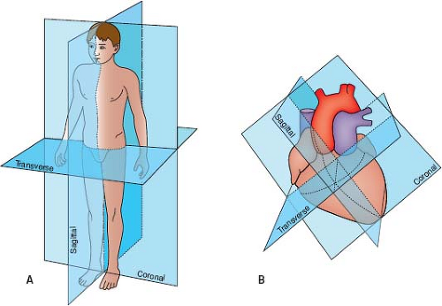 Figure 12.7 A: There are three imaging planes of the body: sagittal, coronal, and transverse. B: There are also three imaging planes of the heart. The cardiac imaging planes are rotated leftward and anterior because the axes of the heart are rotated leftward and anterior relative to the body. |
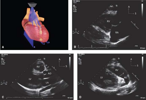 Figure 12.8 The parasternal long-axis sweeps (A) consist of the rightward tricuspid valve view (B), the standard long-axis plane (C), and the leftward pulmonary valve view (D). |
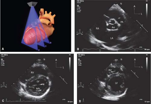 Figure 12.9 The parasternal short-axis sweeps (A) consist of the superior basal view (B), the standard plane at the level of the mitral valve (C), and the inferior papillary muscle view (D). |
Pulsed and Continuous Wave Doppler
Pulsed Doppler causes the transducer to alternately transmit and receive short ultrasound bursts. The time between transmission and reception allows calculation of the depth of the signal or “range-gating” which provides the operator with the Doppler frequency shift at a specific location. A disadvantage with the technique is that the maximal detectable frequency shift is limited—the Nyquist limit (Equation 7: The Basis of Aliasing). However, the Nyquist limit can be extended by shifting the baseline of the spectral display, exchanging to a lower-frequency transducer, or moving to a different imaging plane so that the structure of interest is at a shallower depth if possible. High PRF is a technique in which volleys of pulses of ultrasound are sent before reception of prior pulses. This technique increases the Nyquist limit but causes some range ambiguity.
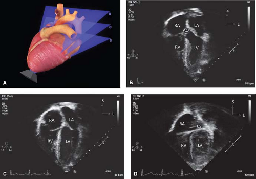 Figure 12.10 The apical sweeps (A) consist of the anterior five-chamber view (B), the standard apical four-chamber view (C), and the posterior coronary sinus view (D). |
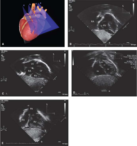 Figure 12.11 The subcostal coronal sweeps (A) consist of the posterior coronary sinus view (B), the standard four-chamber view (C), the anterior left ventricular outflow tract view (D), and the extremely anterior right ventricular outflow tract view (E). |
Continuous Wave Doppler
With the continuous wave Doppler modality, the transducer is continuously transmitting and receiving ultrasound signals. The disadvantage of this process is the absence of range gating, but a major advantage is that the sampling rate is infinite, so there is no longer a limit to the maximal frequency shift. The spectral display consists of a composite of signals with the maximal velocity representing the peak velocity at any depth in the plane of the ultrasound beam. Lower velocities are often visible within the spectral envelope allowing for calculation of “corrected gradients” in which the lower proximal velocity (V1) is subtracted from the higher distal velocity (V2) as is performed for the evaluation of a gradient across an aortic coarctation (23).
Approach to the Pediatric Patient
A cheerful environment is important in relieving anxiety. Television and DVD players can be used to entertain the patients. Warm ultrasound gel also helps in reducing stress. For infants, light dimmers and an infant warmer will facilitate a comfortable environment. Formula should be available for further comforting of infants. Even in a nonthreatening environment, patients over 6 months and under 3 years of age often require sedation. In order to remain compliant
with increasingly strict regulations from the Centers for Medicare and Medicaid Services, many pediatric laboratories are electing to employ anesthesiologists and/or nurse anesthetists for the administration and monitoring of conscious sedation. Monitoring and resuscitation equipment should be available in each room in the event of an adverse reaction or complication.
with increasingly strict regulations from the Centers for Medicare and Medicaid Services, many pediatric laboratories are electing to employ anesthesiologists and/or nurse anesthetists for the administration and monitoring of conscious sedation. Monitoring and resuscitation equipment should be available in each room in the event of an adverse reaction or complication.
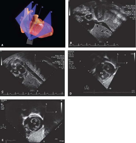 Figure 12.12 The subcostal sagittal sweeps (A) consist of the rightward systemic venous return view (B), the slightly leftward left ventricular outflow tract view (C), the leftward right ventricular outflow tract view (D), and the extremely leftward ventricular view (E). |
Defining Anatomy: Segmental Approach
The echocardiographic examination is performed and the interpretation is presented using a segmental approach (24,25,26,27,28). This requires complete definition of eight features of cardiac anatomy (Table 12.1). This is a two-step process. The first is the proper identification of a structure that requires imaging and recognizing the specific features of each cardiac structure. The second is determining the spatial and physiologic relationships of a properly identified structure to the other structures (both cardiac and noncardiac) in the thoracoabdominal cavity. Accurate morphology can be accomplished definitively only by imaging chamber septal structures. Next, other malformations (e.g., cardiac shunts, valve function) and physiology (biventricular function, chamber sizes, pressure estimates) are described. To ensure that all anatomy and physiology are described, it is helpful during both the performance and interpretation of the examination to imagine the course of a red blood cell traveling through the heart,
beginning in the systemic veins and terminating in the systemic arteries.
beginning in the systemic veins and terminating in the systemic arteries.
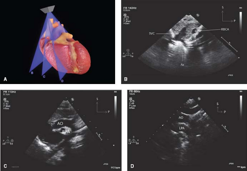 Figure 12.13 The suprasternal long-axis sweeps (A) consist of the rightward superior vena caval view (B), the standard aortic arch view (C), and the leftward left pulmonary artery view (D). |
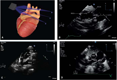 Figure 12.14 The suprasternal short-axis sweeps (A) consist of the very anterosuperior head and neck vessel view (in a patient with right aortic arch and aberrant origin of the left subclavian artery) (B), the anterosuperior vena cava and innominate vein view (C), the standard right pulmonary artery and left atrial view (D), and the posterior descending aorta view (not shown). Even though these imaging planes are defined and illustrated here as discrete planes, the technique of sweeping is a process that allows acquisition of dozens of imaging planes tangential to these. The technique of sweeping through these imaging planes in orthogonal views is critical to understanding the 3-D anatomy. A, anterior; AO, aorta; Az, azygos vein; CS, coronary sinus; INN, innominate vein; IVC, inferior vena cava; L, left; LA, left atrium; LCCA, left common carotid artery; LPA, left pulmonary artery; LV, left ventricle; MV, mitral valve; P, posterior; PA, pulmonary artery; RA, right atrium; RBCA, right brachiocephalic artery; RCCA, right common carotid artery; RPA, right pulmonary artery; RSCA, right subclavian artery; RV, right ventricle; S, superior; SVC, superior vena cava. |
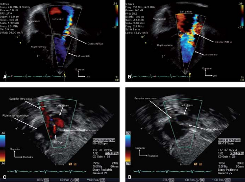 Figure 12.15 Series of four images demonstrating inappropriate and appropriate color aliasing limits during the echocardiographic examination. Throughout an echocardiographic examination the echocardiographer must actively decrease and increase the color aliasing limit depending on the expected velocity of the color jet being interrogated. For example, in evaluating high-velocity jets such as mitral insufficiency, color aliasing limits should be high as in this apical four-chamber view shown in (A) where the velocity limit is 81 cm/s. This provides a clean, crisp, and interpretable display of the mitral insufficiency flow. Inappropriate low color aliasing limit as in (B) (39 cm/s) produces an indistinct display of the mitral insufficiency jet. On the other hand when evaluating a low velocity color jet such as a patent foramen ovale (PFO) the color aliasing velocity should be lower to enhance recognition and display as in the subcostal image (C) where the aliasing velocity is 46 cm/s. If the aliasing velocity is set too high (79 cm/s in this example), detection of the low-velocity PFO jet may be impossible (D). |
TABLE 12.1 Segmental Approach to Defining Cardiac Anatomy by Echocardiography | ||||||||||||||||||||||||||
|---|---|---|---|---|---|---|---|---|---|---|---|---|---|---|---|---|---|---|---|---|---|---|---|---|---|---|
| ||||||||||||||||||||||||||
Abdominal Situs, Cardiac Position, Cardiac Axis
Abdominal situs is best determined from a transverse view of the abdomen below the diaphragm (Fig. 12.16). In this view the positions of the liver and the gastric bubble can be visualized. In patients with abdominal situs solitus, the stomach is on the left and the liver on the right. In patients with abdominal situs inversus, the opposite is true.
The position of the heart in the thoracic cavity is identified most easily from a subcostal coronal view. From the subcostal coronal view, the axis and position of the heart are determined (Fig. 12.17). The normal position of the heart in the left chest is termed levoposition. The normal base to apex axis is termed levocardia. Cardiac position and axis may differ. Mesoposition refers to a cardiac position over the patient’s midline. Dextroposition indicates that the heart lies in the right side of the chest. Dextrocardia refers to the base–apex axis pointing to the patient’s right regardless of the heart’s position in the chest.
Dextroposition with levocardia refers to a condition in which the heart is pushed into the right chest by either a mass in the left chest (e.g., diaphragmatic hernia) or deficiencies in right-sided chest structures. The apex remains pointed to the left; atrial situs, ventricular topology, and great vessel relationships are normal, and cardiac pathology, if present, is not complex. In the two types of dextrocardia, termed “dextroversion” and “mirror-image dextrocardia,” the apex is pointed to the patient’s right. Dextroversion refers to a condition in which there is atrial situs solitus with a rightward-pointing apex. Ventricular inversion (atrioventricular discordance) and associated pathology similar to that seen in congenitally corrected transposition of the great arteries often occurs. Mirror-image dextrocardia is a condition with atrial situs inversus and a rightward-pointing apex. These patients’ anatomy is “mirror image” to that of a patient with levocardia and atrial situs solitus and their anatomy is best appreciated by imagining a mirror placed on a patient with levocardia and situs solitus at the patient’s midline in a sagittal position. In this way, one appreciates that structures that are normally far left (e.g., left ventricle) are in a far right position in a patient with mirror-image dextrocardia. Structures that are closer to the midline (e.g., the superior vena cava [SVC]) are in a midline position in a patient with mirror-image dextrocardia. There may be major and complex pathology associated with mirror-image dextrocardia. However, in situs inversus totalis (a condition in which all body organs are on the contralateral side of the body from which they usually sit), the heart may be completely normal.
When evaluating a patient with any of these three types of dextrocardia, the echocardiographer must maintain left/right convention rather than attempting to make the image look familiar. Specifically, the echocardiographer must remain true to the established echocardiographic convention that the right side of the screen/monitor in the parasternal short axis, apical four-chamber and subcostal coronal view is always the left side of the patient. This convention is maintained by the echocardiographer rotating the transducer so that the “orientation mark” on the transducer is pointing to the patient’s left in these imaging planes. There will be a tendency for the echocardiographer to rotate the transducer to an unusual or atypical position to attempt to make the image look “normal,” but this should be resisted. In some instances, this is problematic because it could reverse the left/right echocardiographic convention.
Venous Return and Atria
Situs
Detailed assessment of the atrial anatomy is an integral part of a complete echocardiogram. Identification of the atrial septum, pulmonary and systemic venous drainage, coronary sinus, and
atrial appendages is key. A definitive conclusion regarding atrial morphology cannot be made by assessment of systemic or pulmonary venous connection or the fact that an atrial chamber is on the patient’s right or left. Atrial situs can be deduced only by evaluation of the atrial appendages and the septal structures.
atrial appendages is key. A definitive conclusion regarding atrial morphology cannot be made by assessment of systemic or pulmonary venous connection or the fact that an atrial chamber is on the patient’s right or left. Atrial situs can be deduced only by evaluation of the atrial appendages and the septal structures.
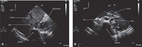 Figure 12.16 Subcostal transverse abdominal views in a patient with abdominal situs solitus (A) and in a patient with abdominal situs inversus (B). With abdominal situs solitus, the liver is on the patient’s right and the stomach is on the left. In abdominal situs inversus, the liver is on the left and the stomach is on the right. A, anterior; Ao, descending abdominal aorta; IVC, inferior vena cava; R, right. |
The atrial appendages are committed to their respective atria and have distinctly different morphology. The right atrial appendage is more anterior, broad-based, and triangular in appearance. It is best visualized in the subcostal sagittal view and the parasternal long-axis view (Fig. 12.18A). The left atrial appendage is relatively posterior in location and has a long and narrow appearance. It is best seen in the parasternal short-axis and apical four-chamber views (Fig. 12.18B).
The unique septal structures of the RA are the embryonic valves—Eustachian and Thebesian—seen in the subcostal coronal and sagittal views. The unique left atrial septal structure is the septum primum, the flap valve of the foramen ovale seen in the apical and subcostal coronal and sagittal views (Fig. 12.19). In atrial situs solitus, the right atrium is located on the right and receives flow from the systemic veins and the coronary sinus. The left atrium (LA) is leftward and typically receives the pulmonary venous return. In heterotaxy syndrome with bilateral right- or left-sidedness and common atrium, the atrial septal structures will not be obvious and atrial situs will be indeterminate or ambiguous.
Systemic Veins and Right Atrium
The innominate veins are identified in the suprasternal short-axis view. Both innominate veins are identified and traced downstream as they join to form the right superior vena cava (RSVC) and followed to its entrance into the heart (Fig. 12.20). The left innominate vein is traced upstream to identify a possible left superior vena cava (LSVC) (Fig. 12.21). A suprasternal notch long-axis view can be swept leftward from the aortic arch to demonstrate an LSVC in a long-axis projection (Fig. 12.22). A high parasternal short-axis imaging plane can demonstrate the anterior and superior lie of the LSVC in relation to the left pulmonary artery (LPA). These maneuvers are particularly important in (a) any patient undergoing surgical repair using cardiopulmonary bypass since a surgeon may have to cannulate both SVCs (when present) in the absence of a left innominate vein and (b) the child with single-ventricle physiology, who will undergo bilateral bidirectional cavopulmonary anastomoses in the presence of bilateral SVC without an innominate vein. In patients with unexplained cyanosis, systemic emboli, or absent innominate
vein without coronary sinus dilation, the presence of an LSVC draining directly into the LA should be investigated. This may require the use of agitated saline contrast that is injected into a left arm vein.
vein without coronary sinus dilation, the presence of an LSVC draining directly into the LA should be investigated. This may require the use of agitated saline contrast that is injected into a left arm vein.
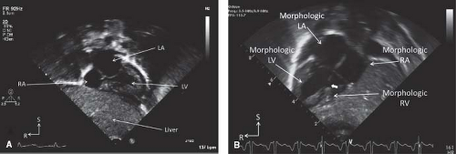 Figure 12.17 Subcostal coronal views of a patient with levocardia (A) and a second patient with dextrocardia (B). In the patient with dextrocardia, the apex of the heart is pointing to the patient’s right. The patient has mirror-image dextrocardia so that the morphologic left atrium (LA) and left ventricle (LV) are on the patient’s right and the morphologic right atrium (RA) and right ventricle (RV) are on the patient’s left. The patient also has a small midmuscular ventricular septal defect (block arrow). R, right; S, superior. |
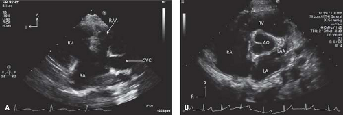 Figure 12.18 Echocardiographic imaging of the atrial appendages. A: The right atrial appendage (RAA) is broad-based and is best seen in the subcostal plane and, as shown here, in the parasternal long view swept rightward. B: The left atrial appendage (LAA) is long and thin and is best seen in the parasternal short axis view. A, anterior; Ao, aorta; I, inferior; LA, left atrium; R, right; RA, right atrium; RV, right ventricle; SVC, superior vena cava. |
The inferior vena cava (IVC) is identified in the subcostal transverse abdominal and subcostal coronal and sagittal views (Fig. 12.16). Identification of interruption of the IVC is important prior to cardiac catheterization. This is apparent in the transverse abdominal view where a large venous vessel immediately posterior to the aorta (the azygos or hemiazygos vein) is seen with notable absence of an intrahepatic IVC anterior to the aorta (Fig. 12.23).
The entrance of the coronary sinus into the RA can be seen in the subcostal coronal and the apical four-chamber views. The size and possible unroofing of the coronary sinus can be assessed in a posterior sweep from the standard apical four-chamber and parasternal long-axis views.
Atrial Septum
The atrial septum is examined in the subcostal coronal and sagittal views. Evaluation for atrial septal defects (ASDs), the size and location, and adequacy of atrial septal rims for possible device closure of secundum-type defects remains important. ASD size, length of atrial septal rims for device anchoring, and total atrial septal length, are evaluated in these two orthogonal planes. The retroaortic (anterior–superior) rim, the tissue between the aorta and defect, can be assessed in the parasternal short-axis view.
Superior and inferior vena caval sinus venosus defects are best seen in the subcostal sagittal view. The transducer should be swept posterior and rightward to investigate possible associated partial anomalous pulmonary venous return. Secundum ASDs are centrally located in the area of the fossa ovalis and are best visualized in the same subcostal imaging planes. The ostium primum defect is related to the crux of the heart and is best seen in the apical four-chamber view. Absence of the atrial septum results in a common atrium and is an extreme form of an ASD. This can also be visualized in the apical and subcostal four-chamber views. A coronary sinus defect is visualized by sweeping the transducer posterior from the standard apical four-chamber view.
Pulmonary Veins and Left Atrium
The pulmonary veins can be identified in multiple imaging planes, including the suprasternal short-axis (Fig. 12.24), parasternal short-axis, and apical four-chamber views. An extreme rightward sweep (tilt right from the SVC, RA, IVC views) in the subcostal sagittal plane should demonstrate the right upper pulmonary vein.
Parasagittal imaging from the bicaval view can show the right pulmonary veins (with a rightward sweep) and the left pulmonary veins (with a leftward sweep) in cross-section as they course into the LA. Color Doppler with a low-velocity aliasing limit can aid in visualizing the individual pulmonary veins (29). Anomalous pulmonary venous connections that typically form a confluence behind the LA should be evaluated from the suprasternal short-axis view (supracardiac drainage), parasternal and apical views (cardiac drainage), and subcostal coronal and sagittal views (infracardiac drainage). Unlike systemic venous anomalies, in which color Doppler demonstrates flow coursing toward the heart, these anomalous pulmonary venous pathways will have low-velocity color Doppler flow coursing away from the heart, often the first sign alerting the echocardiographer to one of these conditions. The LA is best evaluated in the apical four-chamber and the subcostal coronal and sagittal planes. Membranes, such as a supravalvar mitral ring and cor triatriatum, can be identified in the apical four-chamber view. The relationship of these membranes relative to the left atrial appendage is diagnostic. The membrane of cor triatriatum is superior to the LA appendage; however, the membrane of a supravalvar mitral ring may be subtle and is located inferior to the left atrial appendage in the mitral valve funnel itself. This type of membrane may be associated with hypoplasia of the mitral valve annulus.
Parasagittal imaging from the bicaval view can show the right pulmonary veins (with a rightward sweep) and the left pulmonary veins (with a leftward sweep) in cross-section as they course into the LA. Color Doppler with a low-velocity aliasing limit can aid in visualizing the individual pulmonary veins (29). Anomalous pulmonary venous connections that typically form a confluence behind the LA should be evaluated from the suprasternal short-axis view (supracardiac drainage), parasternal and apical views (cardiac drainage), and subcostal coronal and sagittal views (infracardiac drainage). Unlike systemic venous anomalies, in which color Doppler demonstrates flow coursing toward the heart, these anomalous pulmonary venous pathways will have low-velocity color Doppler flow coursing away from the heart, often the first sign alerting the echocardiographer to one of these conditions. The LA is best evaluated in the apical four-chamber and the subcostal coronal and sagittal planes. Membranes, such as a supravalvar mitral ring and cor triatriatum, can be identified in the apical four-chamber view. The relationship of these membranes relative to the left atrial appendage is diagnostic. The membrane of cor triatriatum is superior to the LA appendage; however, the membrane of a supravalvar mitral ring may be subtle and is located inferior to the left atrial appendage in the mitral valve funnel itself. This type of membrane may be associated with hypoplasia of the mitral valve annulus.
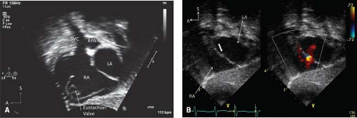 Figure 12.19 Subcostal sagittal views demonstrating a Eustachian valve in (A) and a flap valve (block arrow in B). These unique septal structures are the most reliable method for defining the morphologic right and left atrium (RA and LA), respectively. The color panel of B demonstrates a small left-to-right shunt from the LA to the RA through the patent foramen ovale caused by the flap valve. A, anterior; IVC, inferior vena cava; RPA, right pulmonary artery; S, superior; SVC, superior vena cava. |
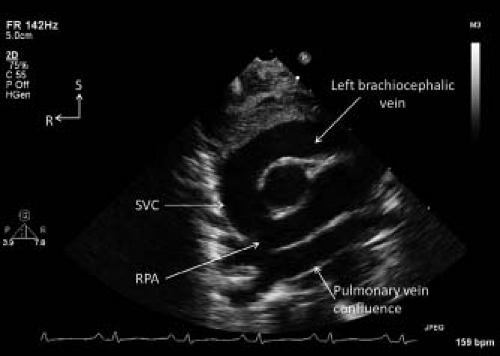 Figure 12.20 Suprasternal notch short axis view demonstrating the left brachiocephalic vein draining into the right superior vena cava (SVC) in a patient with total anomalous pulmonary venous return of the supracardiac type. The pulmonary veins drained to a pulmonary vein confluence immediately superior to the roof of the left atrium. Pulmonary venous flow then continued through a vertical vein, the left brachiocephalic vein, and the SVC resulting in dilatation of the latter two structures. R, right; RPA, right pulmonary artery; S, superior.
Stay updated, free articles. Join our Telegram channel
Full access? Get Clinical Tree
 Get Clinical Tree app for offline access

|