Echocardiographic Assessment of Cardiac Dimensions, Cardiac Function, and Valve Function
Luc L. Mertens
Mark K. Friedberg
Quantification of Chamber Dimensions and Cardiac Structures
Accurate measurements of valves, chambers, and vessels are essential to the diagnosis and management of patients with congenital and pediatric heart disease. The American Society of Echocardiography (ASE) published recommendations for quantification of chamber sizes and function in adults (1,2) and for quantification of cardiac structures in the pediatric population (3). The adult guidelines were recently revised to include three-dimensional (3-D) echocardiography and myocardial deformation imaging (4). One of the important differences between measurements in adult and pediatric patients is the effect of growth or body size on measurements. As dimensions of cardiovascular structures correlate best with body surface area (BSA), indexing the size of cardiovascular structures for BSA has become a commonly used practice. The Haycock formula (BSA [m2] = 0.024265 × weight [kg]0.5378 × height [cm]0.3964) has been recommended for BSA calculation. Correction for BSA is based on the assumption that there is a linear relationship between the cardiac measurement and the BSA. This has been shown to be a simplification as the linear relationship does not hold for the entire spectrum and there is increased variance in the measurements with increasing BSA related to the confounding factors of blood pressure, obesity, and physical activity (5). To overcome this limitation, the use of z-scores has been proposed as a practical alternative (5). Z-scores are based on measurements of cardiovascular structures in a normal population encompassing a wide range of BSA. The z-score represents the number of standard deviations a measurement lies from the mean value at a specific BSA. For instance, z-score of −3.5 for an aortic valve annulus diameter indicates that the value is 3.5 standard deviations below the mean value for that particular BSA. Z-scores for different cardiovascular structures have been published (6,7) but the effect of gender and race on cardiovascular measurements may necessitate establishing normal values based on population mix seen in a specific laboratory.
Detailing the measurement of each individual cardiovascular structure is beyond the scope of this chapter. The reader is referred to recently published guidelines for this purpose (3). In this chapter, the evaluation of cardiac function and chamber quantification are discussed in more detail. In congenital heart disease, chamber quantification can be challenging due to the variable shapes of the ventricles including the right ventricle (RV) and the univentricular heart.
Quantification of the Left Ventricle
The importance of accurately measuring left ventricle (LV) size cannot be overstated. Measurement of LV chamber dimensions at end systole and end diastole (linear dimensions, areas, or volumetric measurements) are used to assess LV remodeling (degree of LV dilation) and function. Measurements of LV wall thickness and mass are important to identify LV hypertrophy.
Linear measurements of LV chamber size and wall thickness have been traditionally obtained using M-mode measurements from the parasternal short- or long-axis views just below the tips of the mitral valve leaflets (Fig. 13.1). M-mode measurements have a very high temporal resolution albeit at the expense of low spatial resolution. It can be difficult to obtain a perpendicular M-mode through the LV resulting in oblique planes that overestimate LV dimensions and increase measurement variability. While the adult ASE guidelines use the parasternal long-axis view to obtain LV measurements, the pediatric ASE guidelines recommended the parasternal short-axis views. If the measurements are not well standardized, M-mode measurements can be highly variable. This was shown by Lipshultz et al. (8) who compared the M-mode measurements made in local echocardiography laboratories and in a core laboratory. This study showed poor agreement between the core laboratory and local laboratory measurements with relatively wide limits of agreement. To overcome some of the problems, the pediatric ASE recommendations suggested using measurements obtained from two-dimensional (2-D) imaging in place of M-mode for LV chamber quantification. Two-dimensional short-axis imaging just
distal to the mitral valve leaflets is recommended (Fig. 13.2) for measuring the internal LV diameter and the inferolateral and septal wall thickness at end diastole and end systole. The downside of this method is the much lower frame rate of 2-D echocardiography. Especially at high heart rates, the identification of the frame representing end systole and end diastole can be more variable. Another limitation is that currently the majority of published normal z-score data are based on M-mode measurements and not on 2-D imaging. Recent data from the Pediatric Heart Network indicated that the LV dimensions could be measured with high reproducibility by both methods and that agreement was high between the two methods (M-Mode vs. 2-D). For calculation of shortening fraction (SF) using M-mode was shown to be more reproducible and it was shown that measurements differed between both techniques (9).
distal to the mitral valve leaflets is recommended (Fig. 13.2) for measuring the internal LV diameter and the inferolateral and septal wall thickness at end diastole and end systole. The downside of this method is the much lower frame rate of 2-D echocardiography. Especially at high heart rates, the identification of the frame representing end systole and end diastole can be more variable. Another limitation is that currently the majority of published normal z-score data are based on M-mode measurements and not on 2-D imaging. Recent data from the Pediatric Heart Network indicated that the LV dimensions could be measured with high reproducibility by both methods and that agreement was high between the two methods (M-Mode vs. 2-D). For calculation of shortening fraction (SF) using M-mode was shown to be more reproducible and it was shown that measurements differed between both techniques (9).
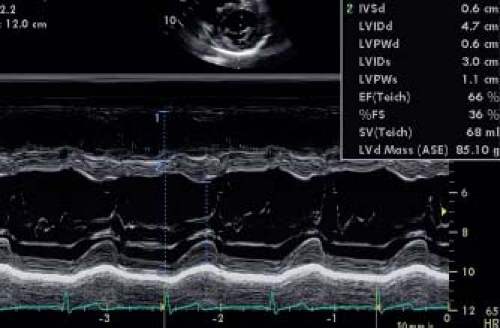 Figure 13.1 M-mode measurements. M-mode measurement is obtained from a parasternal short-axis view of the left ventricle just inferior to the mitral valve leaflets. End-diastolic (at the QRS complex) and end-systolic (at point of minimal diameter) measurements are obtained and fractional shortening and ejection fraction are calculated. EF, ejection fraction; IVSd, interventricular septum at end diastole; LVPWd, left ventricular posterior wall thickness at end diastole; LVIDs, left ventricular end-systolic dimensions; %FS, percent fractional shortening; SV, stroke volume; LVd Mass, left ventricular mass. |
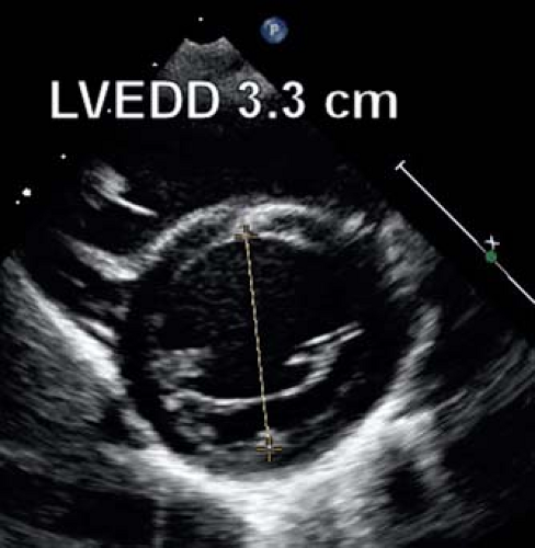 Figure 13.2 Two-dimensional measurement of LV dimensions. The left ventricular end-diastolic dimension (LVEDD) is measured from a parasternal short-axis view just inferior to the mitral valve leaflets. |
2-D and 3-D Techniques
Beyond linear measurements of LV dimensions, it is also possible to calculate LV volumes using either 2-D or 3-D techniques. Two different 2-D techniques (the area-length method and the biplane Simpson’s method) can be used. The area-length method requires measuring the LV major-axis length from a subcostal or apical four-chamber view combined with an area calculation from a subcostal or parasternal short-axis view. The volume is calculated using the formula LV volume = 5/6 × CSA × LV length. As a geometrical formula, this requires a normal ellipsoid LV shape. It becomes more inaccurate in case of spherical remodeling. The biplane Simpson’s method is based on summation of discs and requires delineating the endocardial borders in the apical four-chamber and two-chamber views (Fig. 13.3). Images should be optimized to allow delineation of the endocardium and LV length as suboptimal border detection and foreshortening of the LV are major problems that result in underestimation of the LV volumes. The biplane Simpson’s method is less influenced by ventricular geometry compared with the area-length method and is the method of choice recommended by the adult ASE guidelines. Their accuracy was studied in an adult population where the 2-D biplane Simpson’s method and 3-D imaging for calculating LV volumes were compared to cardiac magnetic resonance imaging (MRI) in patients after acute myocardial infarction (10). This study showed a strong correlation (r = 0.8, p <0.01) between the 3-D echocardiographic and MRI measurements and suggested that the 2-D biplane Simpson’s method was not very accurate and the agreement with MRI was not very strong. The accuracy and reproducibility of these measurements is crucial as LV volumes are used for therapeutic decisions (for instance, LV end-systolic volume in aortic regurgitation). These measurements are also used for calculating ejection fraction (EF) as discussed below. The smaller the LV, the larger is the effect of a measurement error. This is especially important in the borderline LV in patients with aortic stenosis where LV volume calculations may determine a biventricular versus a univentricular treatment approach. For those borderline ventricles accurate calculation of ventricular volumes can be obtained by cardiac MRI.
Calculating volumes based on 2-D images are generally influenced by assumptions of LV shape and geometry. Three-dimensional echocardiography overcomes this problem as full 3-D volumetric data sets can be acquired including the entire ventricle. Most ultrasound systems calculate LV volumes using (semi-) automated
analysis algorithms (Fig. 13.4). This results in improved reproducibility as it eliminates observer bias in determining endocardial borders. Hence, the intra- and interobserver variability of 3-D methods are much lower compared to 2-D-based volumetric calculations. Moreover, 3-D echocardiography is more accurate for determination of LV volumes than 2-D when compared to cardiac MRI (11,12,13). In a pediatric population, 3-D echocardiography has been shown to be the most reliable method for quantification of LV volumes (14). It was included as a recommended method in the most recent revision of the adult ASE guidelines. In adult oncology patients, 3-D echocardiographic assessment of LV ejection fraction was shown to be the most reproducible method. In pediatrics, a limitation of 3-D echocardiography is the lower temporal resolution related to the relative low volume rates. This can be problematic especially in infants with high heart rates. Additionally not every vendor has a high-frequency 3-D probe available, which can limit temporal resolution especially in smaller children.
analysis algorithms (Fig. 13.4). This results in improved reproducibility as it eliminates observer bias in determining endocardial borders. Hence, the intra- and interobserver variability of 3-D methods are much lower compared to 2-D-based volumetric calculations. Moreover, 3-D echocardiography is more accurate for determination of LV volumes than 2-D when compared to cardiac MRI (11,12,13). In a pediatric population, 3-D echocardiography has been shown to be the most reliable method for quantification of LV volumes (14). It was included as a recommended method in the most recent revision of the adult ASE guidelines. In adult oncology patients, 3-D echocardiographic assessment of LV ejection fraction was shown to be the most reproducible method. In pediatrics, a limitation of 3-D echocardiography is the lower temporal resolution related to the relative low volume rates. This can be problematic especially in infants with high heart rates. Additionally not every vendor has a high-frequency 3-D probe available, which can limit temporal resolution especially in smaller children.
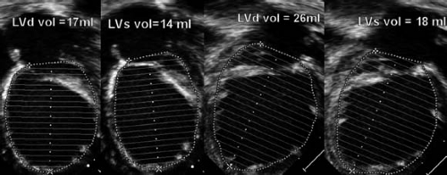 Figure 13.3 Use of biplane Simpson’s rule in calculating left ventricular (LV) volume in patients with severe LV dysfunction. The first two images from the left show the apical four-chamber view in end diastole and end systole, respectively. The next two images are obtained from the apical two-chamber view also in end diastole and end systole, respectively. LV volumes in end diastole and end systole can be calculated. Based on the biplane measurements, the LV ejection fraction in this example is 22%. |
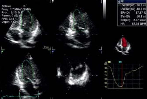 Figure 13.4 Three-dimensional (3-D) echocardiography to assess LV volumes. Three-dimensional echocardiography and (semi-) automated analysis of 3-D volumes is used to measure LV volumetric changes throughout the cardiac cycle. The images represent an apical four-chamber (left upper), an apical two-chamber (right upper), and an apical three-chamber (left lower) cut through the LV volume. The planes through the volumes are illustrated in the right lower panel. On the right of the images, the result of volumetric analysis is shown. LVEDV, left ventricular end-diastolic volume; LVESV, left ventricular end-systolic volume; EF, ejection fraction; SV, stroke volume; CO, cardiac output; HR, heart rate. The lower panel shows the volume–time curve. |
Left Ventricular Mass
Calculation of LV mass can also be important for pediatric patients. In patients with systemic arterial hypertension, LV mass indexed for BSA or height has been shown to correlate well with disease severity and has prognostic implications (15). LV mass is usually calculated using the Devereux formula (LV mass = 0.8 × {1.04[(LVIDd + PWTd + SWTd)3 − (LVIDd)3]} + 0.6 g, where LVIDd is the left ventricular end-diastolic dimension, PWTd is the diastolic posterior wall thickness, and SWTd is the diastolic septal wall thickness) from M-mode or 2-D echocardiography. As LV mass is strongly related to body size, various methods have been proposed to correct LV mass for body size. The best correction in the adult population is to index LV mass in grams by height in meters to the 2.7th power (1). Khoury et al. (16) showed that this correction works well for children >9 years of age but that below that age, there is a significant variation for this index in normal controls. Foster et al. (15) have recently shown that in a pediatric population LV mass-for-height centile curves (and z-scores) are the better method for normalizing LV mass.
The M-mode method only works for concentric hypertrophy as it assumes that the LV walls are homogeneously thickened. This assumption is often inaccurate as even in systemic arterial hypertension the basal LV septum is often thicker than the rest of the LV walls, resulting in overestimation of overall LV mass by the Devereux formula. The formula cannot be used in patients with asymmetric hypertrophic cardiomyopathy. Two-dimensional methods can be used but have higher variability. Recently 3-D methods have been proposed for quantification of LV mass and have been shown to correlate better with MRI measurements of LV mass as they are less dependent on geometrical assumptions (17).
Quantification of the Right Ventricle
Assessment of RV size is even more challenging compared to the LV due to its more complex geometric shape (difficult to describe by a single 2-D measurement or simple geometric formula) and anterior position in the chest (anterior wall in the near field of the ultrasound beam reducing spatial resolution) (18). The ASE published separate guidelines for assessment of the right heart in adults (2) and the pediatric guidelines also contain recommendations for measuring RV dimensions and function (3). Linear measurements have been used to assess RV size. Various measurements obtained from the apical four-chamber view have been proposed (Fig. 13.5). These include measuring RV end-diastolic diameters at the basal
and midcavity levels, RV end-diastolic length, and also end-diastolic and end-systolic RV areas. A problem with these measurements is the lack of normal pediatric data precluding calculation of z-scores. Another problem is that measurements from the apical four-chamber view include only the inlet and the apical portions of the RV and do not account for the RV outlet. Therefore, measurements of the RV outflow tract from either a parasternal short-axis or long-axis view should be made. Z-scores are available for RV outflow end-diastolic dimensions from M-mode, but these mainly reflect RVOT dilation and do not portray remodeling of the remainder of the RV cavity. RV end-diastolic dimension can be measured from this view and z-scores are available for pediatric use. As RV remodeling can affect different parts of the RV differently, this can lead to misrepresentation of RV size if only one dimension is utilized. Based on an RV-centric apical four-chamber view, RV dimensions can be measured at the RV inflow just below the tricuspid valve (RV1) or in the trabecular part (RV2). From this view also RV length can be measured. For RV1 and RV2 no pediatric z-scores are currently available. From the RV-centric apical view RV area can also be measured. In different studies RV end-diastolic area correlated well with measurements of RV end-diastolic volume by MRI (19).
and midcavity levels, RV end-diastolic length, and also end-diastolic and end-systolic RV areas. A problem with these measurements is the lack of normal pediatric data precluding calculation of z-scores. Another problem is that measurements from the apical four-chamber view include only the inlet and the apical portions of the RV and do not account for the RV outlet. Therefore, measurements of the RV outflow tract from either a parasternal short-axis or long-axis view should be made. Z-scores are available for RV outflow end-diastolic dimensions from M-mode, but these mainly reflect RVOT dilation and do not portray remodeling of the remainder of the RV cavity. RV end-diastolic dimension can be measured from this view and z-scores are available for pediatric use. As RV remodeling can affect different parts of the RV differently, this can lead to misrepresentation of RV size if only one dimension is utilized. Based on an RV-centric apical four-chamber view, RV dimensions can be measured at the RV inflow just below the tricuspid valve (RV1) or in the trabecular part (RV2). From this view also RV length can be measured. For RV1 and RV2 no pediatric z-scores are currently available. From the RV-centric apical view RV area can also be measured. In different studies RV end-diastolic area correlated well with measurements of RV end-diastolic volume by MRI (19).
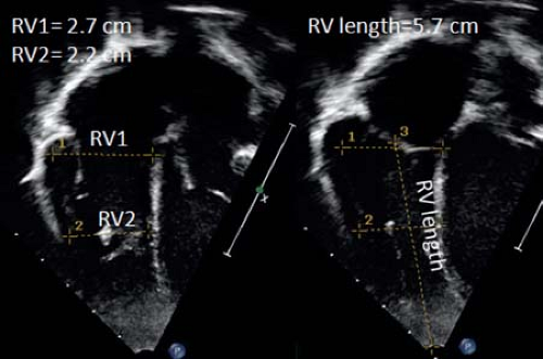 Figure 13.5 Measurement of right ventricular (RV) 2-D dimensions. From the apical four-chamber view, RV width is measured just below the tricuspid valve (RV1) and in the midpart of the RV (RV2). RV length is also measured just after tricuspid valve closure from the mid of the tricuspid valve to the apex of the RV. |
All 2-D-based methods have been shown to underestimate RV volumes when compared to cardiac MRI volumetric calculations. This is mainly due to foreshortening in the 2-D images (it can be difficult to image the true RV apex by echo) and difficulties in defining the endocardial borders. The RV wall is relatively thin (compacted myocardial thickness of 3 to 5 mm in the adult heart) and has coarse trabeculations causing variability in endocardial border definition. In patients after tetralogy of Fallot repair it has been shown that of all 2-D measurements, RV end-diastolic area (RVEDA) correlated the best with RV end-diastolic volume as measured by cardiac MRI (19).
Also for the RV, 3-D echocardiography is a promising tool for assessing RV volumes. Specific analysis software has become available for quantifying RV volumes from 3-D data sets. Full volumetric acquisition can be difficult, especially when the RV is significantly dilated, which limits the feasibility of the 3-D methods. Studies have shown that good quality 3-D data sets can only be obtained in 55% to 75% of patients after tetralogy of Fallot repair (20,21,22). A second problem is that 3-D methods tend to underestimate RV volumes compared to cardiac MRI in patients with congenital heart disease (20,21,22). Studies have suggested that the larger the ventricle, the more important the underestimation. This is probably related to difficult visualization of the endocardial borders related to the coarse trabeculations. Especially at end systole the RV trabeculations can be difficult to identify making the assessment of end-systolic volumes more variable. Also certain anatomical landmarks such as the pulmonary valve and the RV apex can be difficult to identify on 3-D datasets that generally have a lower temporal and spatial resolution.
Quantification of the Univentricular Heart
Assessing chamber dimensions of the univentricular heart can be challenging due to the variable morphology. First, it is important to know whether the dominant ventricle has left, right, or indeterminate morphology. The methods used for measuring the right and left ventricles as described for the biventricular circulation can be applied to the univentricular heart, but “normal” values for the univentricular heart of either LV or RV morphology are unavailable. Moreover, the type of palliation and associated volume loading will influence ventricular size. A shunted single ventricle will generally be larger compared to the same ventricle after total cavopulmonary anastomosis. Margossian et al. (23) demonstrated that when using a biplane Simpson’s method for assessing single LV and RV end-systolic and end-diastolic volumes, good intra- and interobserver agreement can be achieved. Three-dimensional volumes can also be calculated based on full volumetric data sets. It should be noted, however, that the software used for (semi-) automated calculation of LV and RV volumes assumes a specific geometric shape and has not been validated for single ventricles. Soriano et al. (24) used the method of disc summation to measure the volumes of single ventricles. The echocardiographic results were accurate when compared to the MRI results but the method requires extensive off-line manual tracing and processing, limiting its application in clinical practice. More recently Khutty et al. applied 3-D echocardiography for serial measurements of RV volumes in patients with hypoplastic left heart syndrome. He demonstrated a progressive increase in RV end-diastolic volume indexed for BSA after the Norwood operation, which decreased after the bidirectional cavopulmonary anastomosis.
Evaluation of Systolic Ventricular Function
When evaluating systolic function, it is important to consider the different levels (fiber, segment, or ventricle) evaluated by the various functional indices. Overall cardiovascular function can be defined as the delivery of blood to the tissues at a rate commensurate with oxygen consumption. This integrates cardiac and vascular function. To describe cardiac function, a distinction between ventricular and myocardial function can be made. Ventricular function is the pump activity generating an adequate cardiac output at low filling pressures. Myocardial function is the phasic shortening and force generation at the fiber or segmental level, followed by lengthening and force decay. Cardiac function can thus be studied at the level of fiber mechanics, regional or segmental myocardial function, and global pump function (Fig. 13.6). At each level, there is a component of force development and resultant deformational changes. Fiber mechanics describe the relationship between active myocardial fiber force development (contractility) and fiber shortening. The degree of shortening is influenced by the precontraction muscle length (preload) and by the force opposing shortening after the onset of contraction (afterload). The frequency of stimulation will also influence fiber shortening as increased frequency results in increased contractile force development (force–frequency relationship). Echocardiography cannot directly study fiber mechanics. At the level of regional or segmental function, regional force development within a segment will result in regional myocardial deformation. At the segmental level, myocardial force is better described as regional wall stress that is influenced by active contractile force development, pressure, wall geometry (wall thickness, regional wall curvature), and segmental interaction. Current echocardiographic techniques allow quantification of regional myocardial deformation as segment shortening, thickening, and rotation (also called regional myocardial strain or deformation). This allows study of regional ventricular wall mechanics. Global pump function is the product of interaction between the different contractile segments resulting in ventricular pressure generation and, when the outlet valve opens, ejection of blood from the ventricle. On the pump level, ventricular performance is determined by myocardial function (influenced by preload, afterload, and heart rate) and efficient segment interaction (synchronicity of contraction). When interpreting an echocardiographic index of global function, such as EF, it is important to understand that it is influenced by myocardial function and its determinants, synchronicity of contraction, and global ventricular geometry. An EF of 45%, for example, has a completely different implication in a ventricle with severe mitral regurgitation, LV dilation, and left bundle branch block compared to the same EF in a patient with severe aortic stenosis and normal conduction. For interpretation of measurements, it is important to know which physiologic parameters influence the echocardiographic parameters. All too often, measurements are determined to be indices of “contractility,” while there are very few, if any, that are not influenced by loading conditions. Knowledge on the reliability, reproducibility, and accuracy of the methods to assess ventricular function will also influence interpretation of the results. This is especially important for serial evaluation of patients over time.
A program of continuous quality improvement for an echocardiographic laboratory should include regular evaluations of the reliability of the measurements in the individual laboratory (25).
A program of continuous quality improvement for an echocardiographic laboratory should include regular evaluations of the reliability of the measurements in the individual laboratory (25).
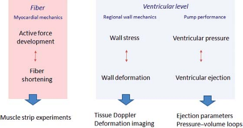 Figure 13.6 Assessment of ventricular function from fiber to pump level. At the fiber level, active force development results in fiber shortening. This relationship can be studied in muscle strip experiments. On the segmental level, regional wall stress is the composite of regional force development and loading on the regional segment. Force development in a segment will result in segmental deformation. Echocardiographically, regional wall motion and deformation can be studied by tissue Doppler and myocardial-deformation imaging. On the pump level, generation of ventricular pressure results in ejection of blood. This can be assessed using ejection parameters like ejection fraction by echocardiography. Invasively this can be studied by pressure–volume loops. |
A wide variety of different echocardiographic parameters and indices has been developed for assessing ventricular function. This in itself indicates that no single parameter adequately provides all the necessary information. The echocardiographer needs to integrate information from different parameters to comprehensively describe systolic function. In this chapter, the most commonly used indices will be discussed with a description of their measurement, reproducibility, accuracy, availability of normal values, and the influence of loading conditions.
One of the most commonly used parameters for assessing LV function is percent shortening fraction (%SF). It is defined as the percentage change in LV dimension from end diastole to end systole. Percent shortening fraction was traditionally measured using M-mode echocardiography from either the parasternal long-axis or short-axis view just below the level of the mitral valve leaflets. The recent recommendations for quantification advise measuring %SF based on 2-D short-axis cuts (either parasternal or subcostal) through the LV. The disadvantage of using 2-D instead of M-mode is the lower temporal resolution. This can be an important problem at higher heart rates, especially in neonates. It can also be difficult to identify end diastole and end systole on 2-D short-axis views. Percent shortening fraction is defined as
where LVEDD is the left ventricular end-diastolic dimension and LVESD is the left ventricular end-systolic dimension. The normal value ranges between 28% and 38%. Values <28% suggest reduced systolic function, while values >38% indicate hyperdynamic function. In most patients, %SF is relatively easy to measure yielding high feasibility. After adequate standardization of acquisition and analysis, variability should be between 10% and 15%. Percent SF has important limitations that should be taken into account when used for clinical decision making. First, %SF measures the apposition of two opposing walls (basal septum and inferolateral wall) as a measure of global systolic function. This assumes that there are no regional differences in wall motion while, in reality, different conditions are associated with regional wall motion abnormalities. In congenital heart disease, hypokinesia and dyskinesia of the interventricular septum occur in the presence of RV volume loading (e.g., large atrial septal defect). This can cause paradoxical septal motion with the septum moving away from the inferolateral wall during systole (Fig. 13.7). Paradoxical septal motion can also
be present in the immediate postoperative (post bypass) period and in the presence of left bundle branch block where maximal systolic motion of the inferolateral wall and septum do not occur simultaneously. All these conditions affect measurement of %SF. In cases of regional myocardial dysfunction, such as after myocardial infarction where the inferolateral and basal septum are not involved, measurement of %SF can overestimate global function. Percent SF is also influenced by preload and afterload and does not directly reflect intrinsic myocardial function. Volume loading will generally increase %SF. An example is the increased %SF in patients with mitral and aortic regurgitation. Pressure loading generally decreases %SF, especially when acute changes occur. A typical example would be an acute increase in arterial blood pressure resulting in an immediate decrease in %SF. This does not reflect an acute decrease in myocardial contractility but rather the increased loading on the heart. A final important limitation is the dependency of the calculation on LV geometry. When hypertrophy of the wall occurs, as happens in the context of chronic arterial hypertension or hypertrophic cardiomyopathy, endocardial changes and chamber dimension changes are influenced by the thickened wall resulting in an overestimation of systolic function.
be present in the immediate postoperative (post bypass) period and in the presence of left bundle branch block where maximal systolic motion of the inferolateral wall and septum do not occur simultaneously. All these conditions affect measurement of %SF. In cases of regional myocardial dysfunction, such as after myocardial infarction where the inferolateral and basal septum are not involved, measurement of %SF can overestimate global function. Percent SF is also influenced by preload and afterload and does not directly reflect intrinsic myocardial function. Volume loading will generally increase %SF. An example is the increased %SF in patients with mitral and aortic regurgitation. Pressure loading generally decreases %SF, especially when acute changes occur. A typical example would be an acute increase in arterial blood pressure resulting in an immediate decrease in %SF. This does not reflect an acute decrease in myocardial contractility but rather the increased loading on the heart. A final important limitation is the dependency of the calculation on LV geometry. When hypertrophy of the wall occurs, as happens in the context of chronic arterial hypertension or hypertrophic cardiomyopathy, endocardial changes and chamber dimension changes are influenced by the thickened wall resulting in an overestimation of systolic function.
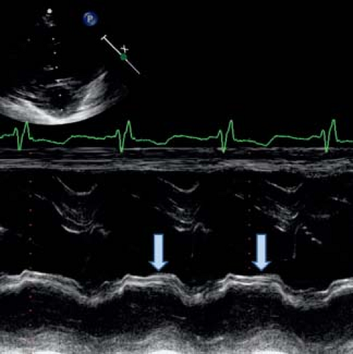 Figure 13.7 Paradoxical motion of the interventricular septum in a patient with a large atrial septal defect. M-mode obtained from a parasternal short-axis view through the dilated RV and smaller LV. The arrows show the motion of the interventricular septum in the direction of the RV in systole. This paradoxical systolic motion makes it impossible to use shortening fraction as a measure for LV systolic function in this setting. |
Ejection fraction is a volumetric measurement reflecting the percentage change in LV volume from end diastole to end systole. It is defined as
where LVEDV is the LV volume at end diastole and LVESV is the LV volume at end systole. LV volumes can be calculated using M-mode echocardiography, 2-D echocardiography, and 3-D echocardiography. As previously mentioned, the recommended 2-D-based methods are the area-length method and the biplane Simpson’s method to quantify EF. Three-dimensional echocardiography has been introduced more recently and has been shown to be more reproducible compared to the biplane Simpson’s method. Normal values for EF range between 54% and 75%. EF is a good parameter for global pump function and takes into account regional wall motion abnormalities. Similar to %SF, the method is load dependent with increased volume loading resulting in higher EF and increased pressure loading decreasing EF.
VCF–End-Systolic Wall Stress Relationship
To overcome the load dependency of the SF and EF measurements, alternative methods have been developed that attempt to correct for the effect of afterload or wall stress. The velocity of circumferential fiber shortening (VCF) measures the velocity of dimensional changes during ejection. Fiber shortening only occurs during ejection and therefore the mean VCF shortening can be calculated as
ET can be calculated from an M-mode of the aortic valve with very high temporal resolution. VCFc should be corrected for heart rate as fiber shortening is influenced by heart rate. The heart rate corrected value can be calculated as
where SF is shortening fraction, RR is R to R interval, and ET is ejection time. The corrected VCFc is relatively insensitive to preload changes but highly sensitive to changes in contractility and afterload. When corrected for afterload, the measurement becomes a good parameter for contractility. The problem is how to clinically define afterload. As “fiber shortening” is calculated by measuring ventricular dimensional changes, the same assumptions can be made to calculate “wall stress.” This is based on the Laplace formula where wall stress in a passive tube is related to ventricular pressure and cavity size and inversely related to wall thickness (σ = (P.r)/2h). Higher ventricular pressure and larger ventricular size increase wall stress while a thicker wall reduces wall stress. Assumptions for both meridional and circumferential wall stress can be derived from M-mode measurements, pressure measurements, and initially, carotid pulse tracing was used to estimate end-systolic wall stress. While peak stress determines the degree of hypertrophy, end-systolic stress is the most important parameter determining systolic shortening (26). The formula that is used to calculate meridional (longitudinal) end-systolic wall stress is
where 1.35 is the conversion factor from mm Hg to g/cm2, Pes is the end-systolic pressure derived from linear interpolation of the dicrotic notch on the pulse trace assigning the systolic blood trace to its peak and the diastolic pressure to its nadir, LVES is the left ventricular end-systolic dimension, and hes is the left ventricular end-systolic wall thickness. Circumferential end-systolic wall stress can also be calculated with the addition of the LV long-axis end-systolic length from the mitral annulus to the LV apex in the apical four-chamber view (L). Thus, circumferential ESWS (g/cm2) = [(1.35)(Pes)(LVES/2hes)] × [1 − (LVES)2/2(L2)]. Both parameters can be obtained from an M-mode echocardiogram of the LV with simultaneous indirect carotid artery pulse trace and blood pressure determination. This makes the method quite cumbersome. Simplified versions include using mean or peak systolic pressures instead of end-systolic estimated pressures (27). Colan et al. (28) found a direct negative correlation between VCFc and end-systolic meridional wall stress. This seems logical as higher afterload can be expected to reduce the velocity of fiber shortening for the same myocardial contractility. The relationship between VCFc and end-systolic wall stress within the normal range has been published (28,29).
Abnormal LV contractility is defined as values for wall stress versus VCFc falling below the normal expected range. In younger children, the linearity of the relationship was questioned and it was shown that wall stress as calculated in the formula misrepresents afterload in children and young adults with abnormal left geometry (30). The relationship between VCFc and wall stress only holds with a normal wall thickness-to-chamber ratio. When this ratio is increased (e.g., hypertrophic cardiomyopathy), meridional wall stress underestimates fiber stress; when the ratio is decreased (e.g., dilated cardiomyopathy), meridional wall stress overestimates fiber stress. The method has been applied in a number of different clinical conditions, especially for the evaluation of cardiac contractility in pediatric patients exposed to anthracyclines. Lipshultz et al. (31) demonstrated that the velocity of fiber shortening versus wall stress is a useful index for following patients after exposure to anthracyclines. Before the wall stress–VCFc relationship (or contractility) becomes abnormal, an increase in wall stress is measured in some patients after chemotherapy, mainly related to a change in wall thickness–chamber dimension ratio (32). Overall, the added benefit of measuring and calculating the VCFc relationship is still uncertain. More advanced calculations have been proposed to calculate midwall shortening and even fiber stress, but, apart from use in research, the clinical applicability and the use of these methods in clinical decision making are currently limited, and clinical decision making is still mainly based on calculation of EF.
Doppler Indices of Ventricular Function
Measurement of EF and %SF provide information on global pump function based on dimensional changes. Derived parameters such as VCFc and wall stress were developed in an attempt to yield information on myocardial and even fiber function.
As all these parameters are based on calculations involving geometrical dimensions, their use in congenital heart disease is limited. As an alternative to measuring geometrical changes, Doppler data have been used to quantify ventricular systolic function. Initially, blood pool velocity measurements were made, and more recently tissue Doppler was introduced to measure the velocity of myocardial motion. The advantage of these methods is that they can be obtained independently of ventricular geometry.
As all these parameters are based on calculations involving geometrical dimensions, their use in congenital heart disease is limited. As an alternative to measuring geometrical changes, Doppler data have been used to quantify ventricular systolic function. Initially, blood pool velocity measurements were made, and more recently tissue Doppler was introduced to measure the velocity of myocardial motion. The advantage of these methods is that they can be obtained independently of ventricular geometry.
One of the proposed blood pool measurements is maximal dP/dt based on a CW Doppler signal obtained through an atrioventricular (AV)-valve regurgitant jet. From invasive pressure measurements, the maximal rate of rise in LV pressure during the isovolumic contraction period (dP/dTmax) has been used as an invasive index for LV function. As Doppler velocity measurements represent pressure gradients, the slope of the CW regurgitant jet represents the speed of pressure rise within the ventricle. Practically, dt is calculated between 1 m/s and 3 m/s; dP between those two time points calculated by the Bernoulli equation is 32 mm Hg. dP/dt can then be calculated by the following formula: dP/dt = 32 mm Hg/time interval in seconds. In the normal LV, dP/dt is 1,200 mm Hg/s or more. The same calculation can be applied to the RV or the univentricular heart. As dP/dt is measured before aortic valve opening, it is independent from changes in afterload but its measurement is influenced by preload changes. As the time interval measured on the Doppler trace is very short and the settings used to obtain the spectral Doppler tracings can be variable, the reliability and accuracy of the method are limited. This confines its use in daily clinical practice.
Assessment of cardiac function by measuring blood flow velocity during ventricular ejection is another logical approach. Doppler signals across the aortic and pulmonary valves can provide timing intervals that are used to assess ventricular function. The time period between the onset of the QRS-complex and the onset of outflow is called the pre-ejection period. This period shortens when the function improves. When the pre-ejection period is corrected for ET, the PEP/ET ratio is a parameter for systolic function. One of the problems is that ET is very sensitive to afterload changes and is heart rate dependent. Moreover, the PEP time interval is short and its measurement influenced by the spectral Doppler settings. A logical next step is to combine inflow and outflow Doppler measurements in the assessment of ventricular function. The myocardial performance index (MPI) was introduced as a nongeometrical index that incorporates both systolic and diastolic time intervals in expressing global ventricular function (33). MPI is defined as
where ICT is the isovolumetric contraction time, IRT is the isovolumetric relaxation time, and ET is the ejection time (Fig. 13.8). When systolic dysfunction is present, ICT will prolong and ET shortens resulting in a prolongation of MPI. When diastolic dysfunction is present, the effect of IRT is dependent on the type of diastolic dysfunction. A relaxation abnormality will increase ICT but elevated filling pressures will have the opposite effect as an increase in left atrial (LA) pressure will shorten IRT. Thus, IRT is strongly dependent on preload and filling pressures while ET is influenced by afterload. Normal MPI values for the LV are 0.35 ± 0.03 and for the RV are 0.28 ± 0.04. MPI has been proposed as an index for global ventricular performance as it incorporates systolic and diastolic function and will also be influenced by loading conditions. MPI has been shown to be a sensitive but not very specific marker of cardiac performance. Nevertheless, in certain diseases like pulmonary hypertension, amyloid heart disease, and pulmonary hypertension, it has strong predictive value (34,35).
Apart from measuring flow velocities, Doppler has also been used for measuring myocardial velocities or tissue Doppler velocities. Tissue velocities are lower than most blood pool velocities but have higher amplitudes. Thus by adjusting Doppler filter settings, tissue Doppler velocities can be selectively measured (Fig. 13.9). Pulsed-wave tissue Doppler was developed first, followed by color tissue Doppler. Pulsed Doppler typically measures velocities in a single segment while color tissue Doppler measures velocities in an entire wall or chamber. While pulsed Doppler measures peak
velocities, color tissue Doppler measures mean velocities. Therefore, color tissue Doppler velocities are approximately 15% to 20% lower than pulsed Doppler velocities. Color Doppler has the advantage of measuring velocities in different myocardial segments simultaneously while pulsed Doppler samples a single segment in a given time. Typically, pulsed tissue Doppler tracings are obtained at the mitral and tricuspid annulus or basal lateral wall and interventricular septal segments to study longitudinal motion in systole and diastole. A typical pattern of myocardial motion comprises an isovolumic spike followed by a systolic velocity wave. The systolic wave can be biphasic, especially in the lateral wall segments. In diastole, early and late (during atrial contraction) diastolic velocities can be measured. Experimental studies have confirmed that, for normal myocardium, changes in segmental systolic velocities are closely linked to changes in contractility but are also influenced by loading conditions. Cardiac translational motion and tethering between segments (a noncontractile segment passively pulled by a normally contracting segment) also influences tissue Doppler velocities. As a Doppler technique, it is, by definition, angle dependent and influenced by machine settings and technical optimization. When the methods are well standardized, tissue Doppler velocities can be measured with reasonable intra- and interobserver variability. Differences between different machines and vendors have been described, especially for color Doppler measurements (36). At present, the use of systolic velocities is limited mainly to the assessment of ventricular dyssynchrony as will be discussed later in this chapter. Diastolic velocities, on the other hand, have become a key component in diastolic function assessment (see below). In the assessment of systolic function, the spike that occurs during the isovolumetric contraction period has been shown to be potentially useful (37). The mean acceleration of this spike, also called myocardial isovolumic acceleration (IVA), can be measured (Fig. 13.10) and has been described to be a relatively load-independent parameter for contractile function. As isovolumic contraction is a short-lived event (30 to 40 ms), calculation of IVA requires obtaining images at high temporal resolution (>200 frames/s) and the reproducibility of the measurements can be difficult if the method is not well standardized. An interesting physiologic characteristic of IVA is its heart-rate dependency. Contractility increases with heart rate as described by the force–frequency relationship and IVA has been shown to be able to study this relationship in normal children and in disease (38). This indeed may be its main application as, due to its heart rate dependency, baseline values of IVA are variable. The measurement thus requires heart rate manipulation with ventricular pacing or exercise testing (38).
velocities, color tissue Doppler measures mean velocities. Therefore, color tissue Doppler velocities are approximately 15% to 20% lower than pulsed Doppler velocities. Color Doppler has the advantage of measuring velocities in different myocardial segments simultaneously while pulsed Doppler samples a single segment in a given time. Typically, pulsed tissue Doppler tracings are obtained at the mitral and tricuspid annulus or basal lateral wall and interventricular septal segments to study longitudinal motion in systole and diastole. A typical pattern of myocardial motion comprises an isovolumic spike followed by a systolic velocity wave. The systolic wave can be biphasic, especially in the lateral wall segments. In diastole, early and late (during atrial contraction) diastolic velocities can be measured. Experimental studies have confirmed that, for normal myocardium, changes in segmental systolic velocities are closely linked to changes in contractility but are also influenced by loading conditions. Cardiac translational motion and tethering between segments (a noncontractile segment passively pulled by a normally contracting segment) also influences tissue Doppler velocities. As a Doppler technique, it is, by definition, angle dependent and influenced by machine settings and technical optimization. When the methods are well standardized, tissue Doppler velocities can be measured with reasonable intra- and interobserver variability. Differences between different machines and vendors have been described, especially for color Doppler measurements (36). At present, the use of systolic velocities is limited mainly to the assessment of ventricular dyssynchrony as will be discussed later in this chapter. Diastolic velocities, on the other hand, have become a key component in diastolic function assessment (see below). In the assessment of systolic function, the spike that occurs during the isovolumetric contraction period has been shown to be potentially useful (37). The mean acceleration of this spike, also called myocardial isovolumic acceleration (IVA), can be measured (Fig. 13.10) and has been described to be a relatively load-independent parameter for contractile function. As isovolumic contraction is a short-lived event (30 to 40 ms), calculation of IVA requires obtaining images at high temporal resolution (>200 frames/s) and the reproducibility of the measurements can be difficult if the method is not well standardized. An interesting physiologic characteristic of IVA is its heart-rate dependency. Contractility increases with heart rate as described by the force–frequency relationship and IVA has been shown to be able to study this relationship in normal children and in disease (38). This indeed may be its main application as, due to its heart rate dependency, baseline values of IVA are variable. The measurement thus requires heart rate manipulation with ventricular pacing or exercise testing (38).
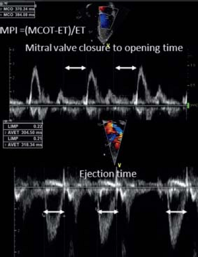 Figure 13.8 Myocardial performance index (MPI). The sum of isovolumetric relaxation and contraction time is calculated by measuring mitral valve closure to opening time (MCOT) and subtracting the LV ejection time (ET). The difference between these two intervals is the isovolumic time. The total isovolumic time divided by the ET gives the MPI. The MCOT is measured on the mitral inflow pattern as shown in the upper part of the picture. The LVET is measured on the aortic outflow as illustrated in the lower part of the figure. |
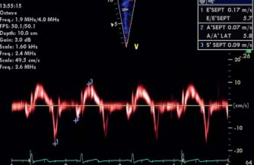 Figure 13.9 Typical longitudinal tissue Doppler tracing obtained in the basal part of the interventricular septum from an apical four-chamber view. Alignment with longitudinal LV motion is extremely important to obtain reliable measurements. Peak systolic velocity (S′) (3), peak early diastolic velocity (E′) (1), and peak late diastolic velocity (A′) (2) are measured. |
Ventricular Strain and Strain Rate
To overcome the problem of cardiac motion and translation as well as to neutralize the effect of intersegmental tethering, myocardial strain imaging was developed. Lagrangian strain is defined as the change in length of a myocardial segment within a certain direction relative to its baseline length. Strain (%) = (Lt − L0)/L0, where Lt is the length at time t and L0 is the length at time zero. Strain rate is the speed at which the deformation occurs and is expressed as %/second. Initially, strain calculations were based on myocardial tissue Doppler velocities by measuring velocity gradients within the myocardium. In the radial direction, for instance, the endocardium moves faster than the epicardium and the gradient between epi- and endocardial velocities correspond to radial strain rate. Temporal integration of the strain rate curve results in the measurement of strain. Tissue Doppler-derived strain measurements are quite cumbersome and require extensive off-line processing with large intra- and interobserver variability if not well standardized. Moreover, tissue Doppler velocities are angle dependent, limiting the measurement of myocardial deformation in certain directions (mainly longitudinal and radial). More recently, it has become possible to measure the strain and strain rate based on speckle-tracking imaging. “Speckles” are gray-scale reflectors within the myocardium and their motion can be tracked in two or three dimensions (Fig. 13.11). The change in distance between the speckles throughout the cardiac cycle can be measured and strain and strain rate derived. The advantage is that this technique is angle independent and most vendors have developed a relatively user-friendly software interface that allows calculation of myocardial strain in different directions (longitudinal, radial, and circumferential). If well standardized, the reproducibility is reasonable but there are significant differences between strain packages from different vendors (39). This seems partially related to where myocardial deformation is measured utilizing different speckle-tracking software. While some programs measure midwall deformation, others measure endocardial or average deformation. This results in different values from different techniques that limit the clinical applicability of the method. Speckle-tracking techniques perform reasonably well for longitudinal strain, but less well for circumferential and especially radial strain. Technical improvements are likely to occur and differences between the different vendors are hopefully to be resolved in the near future through better industry standardization.
The most widely studied parameter has become Global Longitudinal Strain (GLS). This measures the average longitudinal
shortening in the different LV walls as measured from the apical 2-chamber, 3-chamber and 4-chamber views. While limited normative values are available, GLS is considered approximately −20% in a normal adult population (40). Limited normal data are available for the pediatric population (41). In adult cardiology, GLS has been proved a robust and reproducible measurement that can provide additional prognostic information when compared to measurement of EF (42,43). The most recent ASE adult quantification guidelines included GLS measurements (4). The first and probably most important application of strain imaging is quantification of regional myocardial function. This is especially useful when regional wall motion abnormalities are present due to regional myocardial perfusion problems or electromechanical dyssynchrony (Fig. 13.12). Other applications relate to the early detection of myocardial dysfunction, where in certain diseases like Duchenne muscular dystrophy and patients exposed to anthracyclines, a reduction in systolic strain can be observed prior to changes in other cardiac functional parameters. Using strain imaging, a detailed study of myocardial wall mechanics is possible. When interpreting strain data, it should be remembered that strain measurements are influenced by ventricular size and loading conditions. In pediatric heart disease the prognostic value of strain imaging still has to be established and its routine use in clinical practice is still controversial. More recently 3-D speckle tracking have been developed that allow strain quantification of myocardial deformation in different directions based on one single heart beat. This has lower temporal and spatial resolution compared to 2-D speckle tracking.
shortening in the different LV walls as measured from the apical 2-chamber, 3-chamber and 4-chamber views. While limited normative values are available, GLS is considered approximately −20% in a normal adult population (40). Limited normal data are available for the pediatric population (41). In adult cardiology, GLS has been proved a robust and reproducible measurement that can provide additional prognostic information when compared to measurement of EF (42,43). The most recent ASE adult quantification guidelines included GLS measurements (4). The first and probably most important application of strain imaging is quantification of regional myocardial function. This is especially useful when regional wall motion abnormalities are present due to regional myocardial perfusion problems or electromechanical dyssynchrony (Fig. 13.12). Other applications relate to the early detection of myocardial dysfunction, where in certain diseases like Duchenne muscular dystrophy and patients exposed to anthracyclines, a reduction in systolic strain can be observed prior to changes in other cardiac functional parameters. Using strain imaging, a detailed study of myocardial wall mechanics is possible. When interpreting strain data, it should be remembered that strain measurements are influenced by ventricular size and loading conditions. In pediatric heart disease the prognostic value of strain imaging still has to be established and its routine use in clinical practice is still controversial. More recently 3-D speckle tracking have been developed that allow strain quantification of myocardial deformation in different directions based on one single heart beat. This has lower temporal and spatial resolution compared to 2-D speckle tracking.
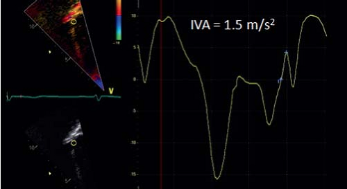 Figure 13.10 Isovolumetric acceleration measured in the RV lateral annulus from an apical four-chamber view. The measurement is performed using color tissue Doppler traced at high frame rates (>180 frames/s). The acceleration of the isovolumetric spike is measured from the baseline to the peak. |
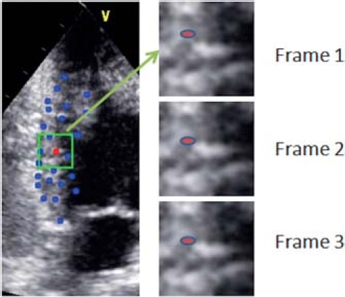 Figure 13.11 Speckle tracking. Speckles are reflectors within the myocardium. They can be tracked throughout the cardiac cycle frame by frame. The motion of the speckles in 2-D or even 3-D space can be used to calculate myocardial deformation. This image is taken from an apical two-chamber view, and speckles within the inferior wall are magnified. The way these speckles move can be traced in 2-D on a frame-by-frame basis as illustrated in the right panels. |
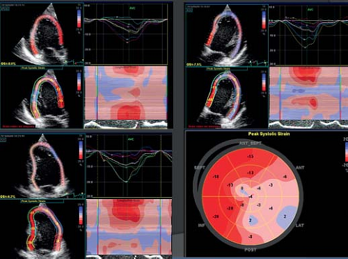 Figure 13.12 Longitudinal LV strain in a 13-year-old girl who developed a myocardial infarction based on abnormal origin of the left coronary artery form the right cusp with posterior looping and intramural course. The left upper panel represents the strain curves obtained from the apical three-chamber view, the left lower panel represents the strain curves obtained from the apical two-chamber view, and the right upper panel represents the strain curves from the apical four-chamber view. Longitudinal strain measurements are significantly reduced in the inferolateral wall segments (light pink and blue areas). The figure on the lower right demonstrates the recommended method for displaying strain data with all 17 cardiac segments portrayed in a bull’s-eye type format. This allows an objective quantification of regional myocardial function. In this patient, the light pink and blue areas in the inferolateral wall segments represent the extent of the myocardial infarction on regional myocardial function. |
Assessment of Right Ventricular Function
The echocardiographic methods to assess ventricular systolic function were mainly developed to assess LV function. The more complex geometry of the RV, its anterior position within the chest, its coarse trabeculations, and its different physiology, make it more difficult to apply these echocardiographic methods for the assessment of RV systolic function (18). Since the normal RV fibers are more longitudinally oriented, longitudinal shortening in the RV is more important than circumferential shortening and radial thickening. The displacement of the basal part of the RV in the direction of the apex during systole is an important contributor to RV ejection. Thus, the study of longitudinal function seems even more important for the RV compared to the LV. While in daily clinical practice assessment of RV function is still largely based on subjective assessment, recent pediatric and adult guidelines include specific recommendations for quantitation of RV function. This is critical for pediatric and congenital heart disease as the RV is often involved in the disease process and assessment of RV function is important for clinical management.
As for the LV, assessment of RV function can be based on the measurement of dimensional changes. Due to the complex geometry however there is no simple method for assessing RV dimensional changes as fractional shortening for the LV. Calculation of RV ejection fraction using the biplane Simpson’s method has been proposed and validated but it can be challenging to image the RV from two orthogonal planes from the apical window. Therefore calculation of percent fractional area change (%FAC) from an apical four-chamber view has become the recommended method. The RV end-diastolic area (RVEDA) and RV end-systolic area (RVESA) are measured and %FAC is calculated as (RVEDA – RVESA)/RVEDA (Fig. 13.13). Care must be taken to include the trabeculations in the RV area. The %FAC has been shown to have a reasonable correlation with MRI EF. One of the limitations is that it can be difficult to trace the endocardial borders related to the coarse trabeculations especially in systole. This results in higher interobserver variability. The %FAC does not represent RV EF well when the RV outflow tract is dysfunctional as is often the case in patients after tetralogy of Fallot repair. In the adult population a %FAC <35% is considered abnormal.
To overcome the exclusion of certain parts of the RV, calculation of RV EF by a 3-D technique would certainly be advantageous. This could be based on volumetric 3-D acquisition or on 2-D-based 3-D reconstruction methods. Software for analysis of RV volumes is available and the volumes obtained using these methods have been shown to correlate well with MRI-derived volumes (Fig. 13.14). However, feasibility is a problem as it can be very difficult to acquire the entire RV volume in a single volumetric data set. Another problem is endocardial border detection that can be challenging in the low-resolution 3-D data sets. Finally, it has been shown that 3-D echo tends to underestimate RV volumes compared to MRI, especially in dilated RVs.
Because longitudinal function is an important component of RV function, different measurements have focused on the assessment of RV longitudinal shortening. The easiest method for assessing longitudinal function is measuring the tricuspid annular planar systolic excursion (TAPSE) by M-mode (Fig. 13.15). It is important to align the cursor with the direction of motion. In adults, the normal excursion is >17 mm. For children, TAPSE is dependent on ventricular size and normal values for children have been published (44). TAPSE is easy to measure and correlates relatively well with EF measurements if there is no significant regional RV dysfunction. It is also influenced by global heart motion and LV-RV interactions. Despite these limitations TAPSE is a potentially useful method for serial follow-up of patients and had prognostic value in certain patient populations.
Systolic tissue Doppler velocities at the tricuspid annulus can also be measured with the same limitations as for the LV. S′-measurements correlate well with parameters of global RV function but is influenced by global heart motion, loading conditions and LV-RV interactions. IVA has been proposed as a more load-independent index of RV contractile function but is heart rate dependent. It has been used to study force–frequency relationships, which requires heart rate manipulation (stress echocardiography or pacing). It is considered more as a research technique rather than a clinical technique.
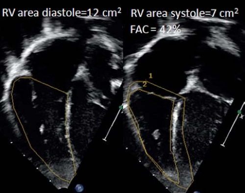 Figure 13.13 Right ventricular fractional area change (FAC). From the apical four-chamber view, the RV is imaged so that the endocardial borders can be tracked as well as possible. The RV area is measured at end diastole and at end systole and FAC is calculated as a percentage. |
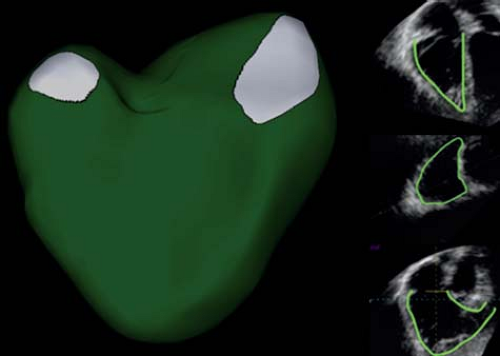 Figure 13.14 Three-dimensional echocardiography to calculate RV volumes. This is based on obtaining a full volumetric data set of the RV and using a semiautomated tracking method to measure RV volume. The left panel represents the reconstructed RV volume with the tricuspid valve on the right and the pulmonary valve level on the left of the volume. The right panels represent the cuts through the volumetric data sets that are traced to reconstruct the RV volume. The right upper is the coronal plane, the middle the transverse plane, and the lower the sagittal plane. |
RV longitudinal shortening can also be quantified using strain and strain rate imaging. Typical RV strain is quantified in the RV free wall from the RV-centric apical four-chamber view. Speckle-tracking echocardiography can be used to measure RV strain but obtaining good tracking in the RV walls can be more challenging due to reverberation artifacts and the relative thin wall of the RV. RV free wall longitudinal strain measurements generally correlate well with global RV EF but in case of regional differences involving the right ventricular outflow tract, the relationship between RV free wall strain and RV EF is less strong (45).
Systolic Function of the Univentricular Heart
With advances in surgical palliation of univentricular congenital heart disease, patients now survive longer and the single ventricle must support both the systemic and pulmonary circulations over many years. Functional evaluation of single ventricles is largely based on subjective assessment and no specific recommendations are available from any professional association. For assessment of a single LV, most of the techniques for assessing the LV in a biventricular circulation can be used. This includes LV EF calculations based on 2-D biplane Simpson’s method. Tissue Doppler measurements and longitudinal strain measurements can also be obtained in this population. In patients after the Fontan operation, while EF is generally within normal range, tissue Doppler velocities and strain measurements tend to be decreased. This is probably related to the chronic volume unloading related to the Fontan surgery and the absence of biventricular interactions. For a single RV, measurements like %FAC, TAPSE, and tissue Doppler can be used. For both the single RV and LV 3-D echocardiography can be used. For all methods interpretation of results is affected by abnormal geometry, ventricular size, and loading conditions.
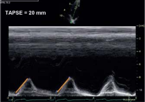 Figure 13.15 Tricuspid annular planar systolic excursion (TAPSE). An M-mode cursor is placed through the tricuspid valve annulus at the RV free wall and longitudinal displacement of the annulus is measured on the M-mode tracing (lines on figure). In this case, TAPSE is 2.7 cm, which is within the normal range (>1.7 cm). |
Ventricular/Ventricular Interaction
In congenital heart, the ventricular–ventricular interactions are important for both systolic and diastolic function assessment. The interventricular septum is an important interface between both ventricles: in RV volume overload, the diastolic flattening of the interventricular septum interferes with LV filling and can influence LV output. In case of pulmonary regurgitation after tetralogy repair, RV dilation has been shown to influence LV filling and pulmonary valve replacement results in better LV filling and improvement in cardiac output (46). Systolic flattening of the interventricular septum is an important phenomenon in RV hypertension that influences LV systolic and also diastolic function (47,48). Description of the septal position in systole and diastole should therefore be part of the assessment of cardiac function. Apart from the influence of the interventricular septum, the epicardial fibers, which are shared between the RV and LV, also influence interventricular cross-talk. In experimental electrically isolated hearts, it has been demonstrated that up to 20% to 40% of the RV systolic pressure and volume output is generated by LV contraction (49,50). How this is important for patients with congenital heart disease needs further exploration. The electrical interreaction between both ventricles is also very important as discussed further in the section on dyssynchrony evaluation.
Assessment of Valve Function
Semilunar Valves and Great Vessels
Quantitative Morphometric Evaluation
Quantitative anatomic assessment of the proximal great vessels and their branches is important in a number of circumstances. It is routine to perform a quantitative evaluation of the aortic structures from the level of the valve annulus through the distal aortic arch. Evaluation of the aortic root itself consists of 2-D assessment of the aortic annular dimension, dimension of the aorta at the level of the sinuses of Valsalva, and dimension of the sinotubular junction, ascending aorta, proximal and distal transverse aortic arch, and aortic isthmus. In general, 2-D axial resolution is superior to lateral resolution. Therefore, aortic root dimensions are best assessed in the parasternal long axis with the proximal ascending aorta and aortic root perpendicular to the ultrasound beam. Different techniques for measuring the aortic root have been proposed and when using normal data, it is important to know which technique was used to establish the reference values. Measurements can be obtained during early to midsystole as suggested by the pediatric guidelines (3), but most of the normal reference papers have used diastolic measurements of the aortic root. Roman et al. (51) and the more recent paper by Gautier et al. (52) both measured the aortic root at end diastole and also used a leading edge to leading edge technique, which means that they included the anterior wall of the aorta in the measurement but not the posterior wall. The alternative technique is to measure the aortic root between the anterior and posterior inner edges. This is the method used in other imaging modalities like cardiac MRI and cardiac CT and the increased image resolution of echocardiography should allow use of the inner-edge technique.
The aortic valve is magnified in the parasternal long-axis view and the annulus measured from the inner edge of the proximal valve insertion hinge point within the arterial root to the inner edge of the opposite hinge point (Fig. 13.16). The sinus of Valsalva and sinotubular junction are also measured from the parasternal long-axis view. To visualize the aortic root and ascending aorta, it may be necessary to move the transducer one or two intercostal spaces higher (high left parasternal view). The ascending aorta is measured at the level where it crosses the right pulmonary artery. Imaging of the transverse arch and isthmus is usually done in long-axis images of the aortic arch from the suprasternal notch window. Measurements should be performed at the level of the proximal transverse arch (between the innominate and left carotid arteries), the distal transverse arch (between the left carotid and left subclavian arteries), and the aortic isthmus (the narrowest segment distal to the left subclavian artery).
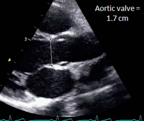 Figure 13.16 Measurement of the aortic valve annulus. A zoomed parasternal long-axis view of the aortic valve is used. The measurement is performed in early systole. The measurement is made at the aortic valve hinge points. |
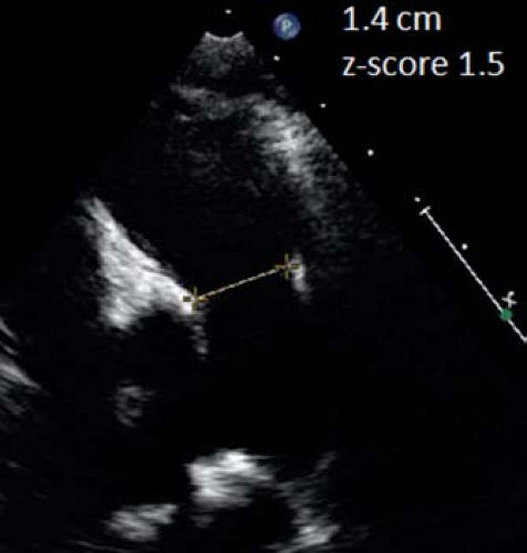 Figure 13.17 Pulmonary valve measurement. In this parasternal short-axis view, the pulmonary valve annulus is measured at the hinge point of the valve leaflets in early systole. |
The pulmonary valve is best measured from the parasternal long-axis outflow view, although it can also be measured from the parasternal short-axis view (lower resolution) (Fig. 13.17).
The main pulmonary artery can be measured between the sinotubular junction and the bifurcation. The proximal right pulmonary artery is best measured from the suprasternal view where it crosses behind the aorta. The left pulmonary artery is best measured from the suprasternal or ductal view.
Semilunar Valve Stenosis
Prior to measuring gradients, the level of obstruction needs to be determined by 2-D and color Doppler imaging. Subvalvar and supravalvar stenosis should be excluded. The severity of aortic and pulmonary valve stenosis in pediatric heart disease is based on Doppler measurement of the peak and mean transvalvular gradient. As with all Doppler assessments, interrogation of transvalvular flow jets should be performed with an angle of insonation as parallel to the direction of flow as possible to minimize underestimation of the valve gradient. As such, aortic valve gradients are most accurately assessed from either the apical window or from a high right parasternal window, with the ultrasound plane angled inferiorly toward the ascending aorta (Fig. 13.18). Suprasternal windows can also be helpful. For the pulmonary valve, the parasternal short- and long-axis views can be used and in infants and smaller children, subcostal imaging can be useful. The peak instantaneous Doppler velocity is measured and the gradient calculated using the Bernoulli equation. This is different from the peak-to-peak gradient measured in the cardiac catheterization laboratory by pullback of the
catheter across the valve. The peak instantaneous pressure gradient is calculated from the peak instantaneous flow velocity that occurs across the semilunar valve at a single time point in systole. When peak-to-peak gradients are measured by pullback of the catheter in the cardiac catheterization laboratory, the gradient is expressed as the difference between the peak pressure upstream of the valve (or point of obstruction) and peak pressure proximal to the valve, which does not occur simultaneously in the cardiac cycle. The peak-to-peak gradient measured by echocardiography will often be higher compared to the peak-to-peak gradient measured by catheterization. The mean aortic gradient can be obtained by tracing the flow profile. Mean gradients correlate better with peak-to-peak gradients obtained in the catheterization laboratory. For the pulmonary valve, the peak instantaneous gradient correlates better with the peak-to-peak gradient on pullback—and this explains why for assessing severity of pulmonary valve stenosis, the peak instantaneous gradient is used—while for the aortic valve, the mean gradient is considered to better correlate with the peak-to-peak gradient.
catheter across the valve. The peak instantaneous pressure gradient is calculated from the peak instantaneous flow velocity that occurs across the semilunar valve at a single time point in systole. When peak-to-peak gradients are measured by pullback of the catheter in the cardiac catheterization laboratory, the gradient is expressed as the difference between the peak pressure upstream of the valve (or point of obstruction) and peak pressure proximal to the valve, which does not occur simultaneously in the cardiac cycle. The peak-to-peak gradient measured by echocardiography will often be higher compared to the peak-to-peak gradient measured by catheterization. The mean aortic gradient can be obtained by tracing the flow profile. Mean gradients correlate better with peak-to-peak gradients obtained in the catheterization laboratory. For the pulmonary valve, the peak instantaneous gradient correlates better with the peak-to-peak gradient on pullback—and this explains why for assessing severity of pulmonary valve stenosis, the peak instantaneous gradient is used—while for the aortic valve, the mean gradient is considered to better correlate with the peak-to-peak gradient.
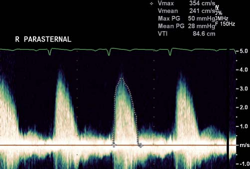 Figure 13.18 Continuous wave Doppler tracing obtained in patient with aortic stenosis from the right parasternal window with the patient in a right lateral decubitus position. This position and view frequently affords the best Doppler alignment with the aortic stenosis jet. Peak gradient as well as mean gradient are measured on the tracing. |
When interpreting gradients, it is important to consider the ventricular function. A low gradient across the aortic valve with poor LV systolic function can result in underestimation of the severity of stenosis. Any factor causing increased flow in the LV outflow such as hyperdynamic ventricular function, anemia, and associated aortic insufficiency will result in higher gradients. As cardiac catheterization is often performed under general anesthesia, it is not unusual to find significant differences in the gradient before and after induction of general anesthesia. Another factor influencing the assessment of Doppler gradients in children is the pressure recovery phenomenon. Potential energy is converted into kinetic energy when blood accelerates across the vena contracta. Some of this energy dissipates into heat related to turbulence and viscous losses. Some of the kinetic energy reconverts to potential energy, resulting in pressure increase distal to the stenosis. This phenomenon is more important when the aorta is smaller and results in overestimation of pressure gradients. Other formulas have been proposed that allow better prediction of the catheter peak-to-peak gradient, but have not been extensively validated.
If there is uncertainty regarding the importance of a semilunar valve stenosis, it can also be useful to try to estimate right or LV pressure, using AV valve regurgitation. RV systolic pressure can be assessed by measuring the peak velocity of the tricuspid regurgitant jet. The RV systolic pressure = 4 (TR peak velocity)2 + estimated right atrial (RA) pressure. In general, RA pressure is estimated to be 5 mm Hg unless there is clinical evidence of elevated RA pressure. LV systolic pressure can be estimated based on the mitral regurgitant jet using the same formula. It can, however, be more difficult to estimate LA pressure.
Calculation of Valve Areas
Because of the aforementioned factors influencing calculation of pressure gradients, estimation of aortic valve area is recommended in the adult patient with aortic stenosis (53). The recommended method to measure aortic valve area is the continuity equation. This equation, based on the principle of conservation of mass, states that with no net loss of fluid from the system, the volumetric flow at area A must be equal to the volumetric flow at area B. The equation is therefore stated as
where A is the cross-sectional area of either position 1 or 2, and V is the mean velocity of the modal spectral profile at either position 1 or 2.
As the mean flow velocity, V, equals the velocity–time integral of flow divided by the ET, and as the ETs across both areas 1 and 2 are essentially the same, the continuity equation is further simplified as follows:
where VTI is the velocity–time integral of flow across either area 1 or 2.
The continuity equation is most frequently used in clinical studies to estimate the effective aortic valve area in the setting of aortic stenosis. By rearranging the continuity equation, the effective valve area of a stenotic aortic valve can be solved for as follows:
where AAOV is the cross-sectional area of the effective aortic valve orifice, ALVOT is the cross-sectional area of the LV outflow tract (LVOT), solved by measuring the diameter of the LVOT in the
parasternal long-axis view, VTILVOT is the velocity–time integral of flow across the LVOT, and VTIAOV is the velocity–time integral across the stenotic aortic valve.
parasternal long-axis view, VTILVOT is the velocity–time integral of flow across the LVOT, and VTIAOV is the velocity–time integral across the stenotic aortic valve.
Using the continuity equation, it has been demonstrated that the aortic valve areas calculated in children by Doppler correlate well to aortic valve areas calculated by the Gorlin equation on cardiac catheterization, although Doppler methods tend to underestimate catheter areas slightly (54). In normal children and adolescents, it has been shown that aortic valve area indexed to BSA is approximately 1.33 cm2/m2 (55), which is very close to values obtained in normal adults (56). Due to the potential inaccuracies in measurement of the LV outflow tract and the larger error associated with the assumption that the outflow tract is circular, the calculation of the valve area is not widely applied in pediatric echocardiography. Direct planimetry by 2-D and 3-D methods have been proposed but due to doming, funnel-type opening of the valve leaflets, the actual orifice is difficult to identify and true en-face views of the valves are difficult to obtain. Three-dimensional methods could potentially help to resolve this problem but have not been validated in pediatric cardiology.
Aortic Valve Insufficiency
Isolated aortic regurgitation in the pediatric population is relatively uncommon, but it can be seen, particularly in children with bicuspid aortic valves. More often, aortic regurgitation is seen in conjunction with an abnormal aortic valve that features both aortic stenosis and insufficiency. Evaluation of neoaortic insufficiency, however, can be important following aortic valve replacement by pulmonary autograft (Ross procedure), in hypoplastic left heart syndrome following a Norwood reconstruction or following an arterial switch operation in transposition of the great arteries. In general, methods for assessing aortic regurgitation can be divided into (a) assessment of LV end-diastolic and end-systolic dimensions and volumes (see section above) and (b) assessment of the aortic regurgitation severity using Doppler methods.
Hemodynamically significant aortic regurgitation results in enlargement of the LV with an increase in LV end-diastolic dimensions and volume. In the case of preserved LV function, hyperdynamic LV function is often associated with LV dilatation (Frank–Starling relationship) causing the LV end-systolic dimension to remain low. With progressive aortic regurgitation and associated LV dysfunction, the end-systolic dimensions (and volume) will increase. In adult patients, it has been proposed in the 2014 ACC/AHA Valve Guidelines that aortic valve replacement or repair be undertaken for end-systolic dimension >50 mm or 25 mm/m2 to protect against irreversible myocardial damage and risk of sudden death (57). In children, a z-score of >4.0 has been suggested but this is not based on good prospective data. Due to the effect of loading conditions on most echocardiographic functional parameters, it is uncertain which parameter best detects early ventricular dysfunction.
Apart from assessing the effect of chronic regurgitation on the LV size and function, the severity of aortic regurgitation needs to be assessed. Different methods should be combined for a comprehensive assessment. Pulsed-wave Doppler flow patterns in the distal aortic arch and descending aorta can be used to assess severity of aortic regurgitation. Significant aortic regurgitation results in holodiastolic flow reversal in the distal aortic arch up to the descending aorta at the level of the diaphragm (Fig. 13.19). Color Doppler interrogation of the aortic insufficiency jet itself can also be performed and various measurements made on the color Doppler images: (a) Jet width or cross-sectional area. This is measured immediately below the aortic valve, within 1 cm of the valve (for adults). In the long-axis view, jet width relative to the LV outflow tract dimension can be measured. From the parasternal short-axis view, the cross-sectional area relative to the LV outflow tract area can be measured. The criteria to define severe AR are ratios of >65% for jet width and >60% for jet area. This has not been well validated in pediatric aortic regurgitation. (b) Measurement of the vena contracta. The vena contracta is defined as the smallest diameter of flow at the level of the aortic valve, immediately below the region of flow convergence. It is different from the jet width that is measured in the LVOT. A vena contracta >0.6 cm in adults is associated with severe AI but no data are available for children. (c) CW Doppler of the regurgitant jet. The best signals are usually obtained from the apical windows. The most commonly used parameter is the pressure half-time of the aortic insufficiency velocity profile (the time required for the initial peak gradient between aorta and LV to decrease by half). A pressure half-time >500 ms usually indicates mild AR, whereas a value <200 ms is consistent with severe AR. The problem with this measurement is that it is influenced by LV end-diastolic pressure and the presence of diastolic dysfunction. Increased end-diastolic pressure will shorten the duration of regurgitant flow.
Regurgitant volume, regurgitant fraction, and effective regurgitant orifice area can all be directly estimated by a combination of Doppler and 2-D echocardiography. Estimation of regurgitant volume and EROA can also be done using color flow Doppler imaging of the regurgitant jet and the proximal isovelocity surface area (PISA). These methods are rarely applied in pediatric echocardiography laboratories due to high variability and inadequate validation.
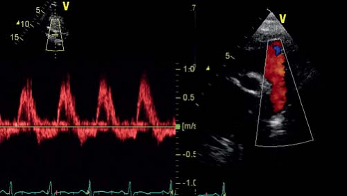 Figure 13.19 Patient with severe aortic regurgitation. Holodiastolic backflow in the abdominal aorta is shown on the pulsed Doppler tracing in the abdominal aorta. Color Doppler also shows the diastolic retrograde flow in the descending thoracic aorta. |
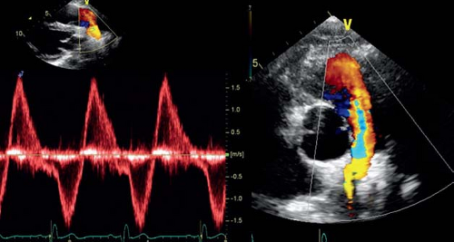 Figure 13.20 Severe pulmonary regurgitation after TOF repair. A wide regurgitant jet can be seen in the main pulmonary artery originating distally from the right pulmonary artery. The Doppler pattern shows the protomesodiastolic duration of the jet with its termination late in diastole. |
Pulmonary Valve Regurgitation
In theory, all the techniques described for aortic valve regurgitation could be used to assess severity of pulmonary valve regurgitation. In practice, pulmonary valve regurgitation is most commonly graded using color Doppler flow. Flow reversal in the pulmonary artery is assessed and, in general, the presence of flow reversal in the distal branch pulmonary arteries is seen in severe pulmonary regurgitation (Fig. 13.20). Jet width relative to the RVOT dimension can be measured. Finally pressure half-time and duration of the pulmonary regurgitant flow relative to the total time of diastole can be used to quantify severity of pulmonary regurgitation. These, however, are influenced by RV end-diastolic pressure. The impact of pulmonary regurgitation on RV dimensions and function can be assessed as discussed in the section on RV volume and function. Based on cardiac MRI data, an RV end-diastolic volume between 150 and 170 mL/m2 has been proposed as an indication for pulmonary valve replacement.
Atrioventricular Valve Size and Function
Quantitative Morphometric Evaluation
The annuli of the tricuspid and mitral valves have an elliptical and saddle-like shape and are best measured from the apical four-chamber view and parasternal long-axis view (Figs. 13.21 and 13.22). The
diameters of the valves should be measured in early diastole at the frame after maximal excursion of the leaflets from inner edge to inner edge at the hinge points of the leaflets. The values should be expressed as z-scores. The area of valves can be calculated using the formula of an ellipse. Planimetry based on 2-D or 3-D images can also be used to measure AV valve size. Tricuspid and mitral valves annular sizes are important in valve disease as well as in the assessment of ventricular size.
diameters of the valves should be measured in early diastole at the frame after maximal excursion of the leaflets from inner edge to inner edge at the hinge points of the leaflets. The values should be expressed as z-scores. The area of valves can be calculated using the formula of an ellipse. Planimetry based on 2-D or 3-D images can also be used to measure AV valve size. Tricuspid and mitral valves annular sizes are important in valve disease as well as in the assessment of ventricular size.
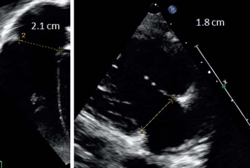 Figure 13.21 Measurement of the tricuspid valve in two planes. Left panel shows the apical four-chamber view and right panel the parasternal long-axis inflow view. The valve is measured in diastole with the leaflets open. |
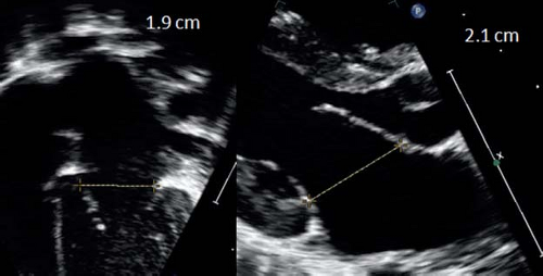 Figure 13.22 Measurement of the mitral valve in two planes. Left panel shows the apical four-chamber view and right panel the parasternal long-axis view. The valve is measured in diastole with the leaflets open. |
Mitral or Tricuspid Stenosis
Isolated mitral or tricuspid valve stenosis are rare congenital lesions. Echocardiography is used to define the mechanisms contributing to valvar narrowing and requires a detailed description of the supravalvar region (supravalvular ring), leaflets (thickened, reduced mobility), chordae (short chordae in case of arcade mitral valve), and papillary muscles (parachute mitral valve). In patients with AV valve stenosis, the Doppler flow will usually be turbulent and its velocity elevated. The early peak velocity can be increased in cases of elevated filling pressures associated with LV diastolic dysfunction, which should be distinguished from mitral valve stenosis. The best method to assess AV-valve stenosis severity is by calculation of mean gradients using the mitral or tricuspid inflow signal (Fig. 13.23). For the tricuspid valve, there can be considerable influence of respiration on the inflow gradient with an increasing gradient during inspiration and decreasing gradient during expiration. Therefore, the gradient should be averaged over at least three to five cardiac cycles. Heart rate and associated AV-valve regurgitation will also influence the calculated mean gradient. The severity of mitral valve stenosis can also be assessed by calculating the pressure half-time (the time needed for the peak early diastolic pressure to decline by 50%). A pressure half-time <60 ms is
normal. A pressure half-time (T1/2) >100 ms is indicative of significant mitral stenosis. Based on mitral valve pressure half-time, mitral valve area can be measured based on the formula (220/T1/2). However, this calculation is not usually applicable in children due to higher heart rates influencing T1/2. Effective orifice size can also be measured by the continuity equation, although again, this is more problematic in children. Direct planimetry based on 2-D or 3-D short-axis views of the mitral valve has been proposed but has not been well validated. Therefore, in practice, the most commonly used method is calculation of the mean gradient across the valve. The presence of an atrial septal defect/patent foramen ovale can lead to atrial decompression with lowering of atrial pressures resulting in a reduction of the gradient across the mitral valve. Therefore, in addition to the heart rate, the presence of an atrial communication should also be noted.
normal. A pressure half-time (T1/2) >100 ms is indicative of significant mitral stenosis. Based on mitral valve pressure half-time, mitral valve area can be measured based on the formula (220/T1/2). However, this calculation is not usually applicable in children due to higher heart rates influencing T1/2. Effective orifice size can also be measured by the continuity equation, although again, this is more problematic in children. Direct planimetry based on 2-D or 3-D short-axis views of the mitral valve has been proposed but has not been well validated. Therefore, in practice, the most commonly used method is calculation of the mean gradient across the valve. The presence of an atrial septal defect/patent foramen ovale can lead to atrial decompression with lowering of atrial pressures resulting in a reduction of the gradient across the mitral valve. Therefore, in addition to the heart rate, the presence of an atrial communication should also be noted.
Stay updated, free articles. Join our Telegram channel

Full access? Get Clinical Tree


