Chapter 14 Computed Tomographic Angiography

Volumetric data acquisition with multidetector computed tomography (MDCT) has enabled the development of computed tomographic angiography (CTA), a diagnostic modality that has clearly revolutionized the diagnosis of vascular disorders. Adequate imaging of the peripheral vascular system during a single acquisition and a single injection of contrast medium became feasible with the introduction of a 4-slice computed tomography (CT) system with a 0.5-second gantry rotation (thinnest collimation 4 × 2.5 mm) in 1998.¹ The introduction of 8-slice CT in 2000 enabled shorter scan times, but did not yet provide improved longitudinal resolution (thinnest collimation 8 × 1.25 mm). The introduction of 16-slice CT made it possible to routinely acquire substantial anatomical volumes with isotropic sub-millimeter spatial resolution.² Computed tomographic angiography scans of the peripheral vasculature could now be routinely acquired with 16 × 0.625 mm or 16 × 0.75 mm collimation, which provided the level of resolution required to investigate small-vessel involvement (<1 mm).

The 64-slice CT systems introduced in 2004 were the next major advance, when two different scanner concepts were introduced by different vendors. The volume concept pursued by General Electric, Philips, and Toshiba aimed at a further increase in volume coverage speed by using 64 detector rows instead of 16, without changing the physical parameters of the scanner compared to the 16-slice version. The resolution concept pursued by Siemens used 32 physical detector rows in combination with double z-sampling, a refined z-sampling technique enabled by a periodic motion of the focal spot in the z-direction to simultaneously acquire 64 overlapping slices. The goal was pitch-independent increase of longitudinal resolution and reduction of spiral artifacts.

With the most recent generation of CT systems, further increases in detector arrays allow increases in volume coverage and acquisition of large volumes in single heartbeats. Although clearly advantageous in coronary imaging, these have also provided advantages for vascular imaging, including arterial phase imaging and diagnosis of vascular disorders such as dissection and arteriovenous malformations (AVMs).

This chapter discusses the basic principles of MDCT and provides an overview of its application in vascular diseases. Image interpretation methods have also evolved, with routine postprocessing methods for image display, analysis, and quantitation. These methods will be discussed, as well as the strengths and weaknesses of CTA, including radiation dose concerns.

Fundamentals of Computed Tomography Imaging

Major Components of a Computed Tomography Scanner

The major components of a CT scanner are an x-ray tube and generator, a collimator, and photon detectors. These components are mounted on a rotating gantry where the x-ray tube produces the x-rays necessary for imaging. The pre-detector collimator helps shape the x-ray beams that emanate from the x-ray tube in order to cut out unnecessary radiation. The detectors consist of multiple rows of detector elements (>900 elements per row in current scanners) that receive x-ray photons that have traversed through the patient, with the post-detector collimators preventing backscatter, which degrades image quality. Newer scanners have as many as 320 detector rows, and the width of each detector (“detector collimation”) has decreased from 2.5 mm in 4-slice systems to 0.5 mm. The most important benefit of increasing the detector rows is increased coverage per gantry rotation (a 320-row detector CT with a detector width of 0.5 mm will have 160 mm z-axis coverage). The submillimeter detector width improves spatial resolution in the z-axis, while increased coverage shortens scan time. Each detector element contains radiation-sensitive solid state material (e.g., cadmium tungstate, gadolinium oxide, gadolinium oxysulfide) that converts the absorbed x-rays into visible light.³ The light is then detected by a silicone photodiode, amplified, and converted into a digital signal.

Gantry rotation time determines the temporal resolution of the images, with older scanners having a rotation time of 0.75 seconds, and more contemporary scanners a rotation time of 0.33 seconds.² The temporal resolution of a single source scanner, one x-ray generator mounted on the gantry, is slightly higher than half the time it takes for the gantry to rotate 360 degrees. Thus a 0.33-second gantry rotation will effectively provide a temporal resolution of 0.17 seconds. With a dual-source scanner, two x-ray generators mounted on the gantry, the temporal resolution will improve by a factor of two.

Computed Tomography Attenuation Data for Image Reconstruction

Computed tomography measures the local x-ray attenuation coefficients of the tissue volume elements, or voxels, in an axial slice of the patient’s anatomy. The attenuation coefficients are then translated into grayscale values (CT value) of the corresponding picture elements (pixels) in the displayed two-dimensional (2D) image of the slice. The numerical CT value is normalized to the attenuation properties of water and is reported as Hounsfield units (HU). Pixel values are stored as integers, in the range − 1024 HU to 3071 HU, corresponding to 4096 different grayscale values. By convention, water = 0 HU, and air = − 1000 HU and is independent of the x-ray spectrum. The CT values of human tissue, however, depend on the x-ray spectrum. In general, lung and fat have negative CT values, muscle has a positive HU, and bone has rather large CT values up to 2000 HU. Administration of iodine contrast agent increases the CT value, with contrast-filled vessels typically having CT values in the range 200 HU to 600 HU. In most cases, contrast-filled vessels can be easily differentiated from the surrounding tissue, which does not exceed a CT value of 100 HU, with the exception of bone.

This easy threshold-based differentiation is the basis for CTA and related image postprocessing techniques. The gantry rotates around the patient, collecting attenuation data from different angles. The attenuation coefficient also varies depending on the energy of the photons (measured in kiloelectron volts [keV]) that pass through them. The measured intensity of photons at the CT detector is related to the photon flux (number of photons) coming through the x-ray tube and that detected at the detector elements. Consequently, as the attenuation of the tissue increases, the fraction of photons detected at the detector element decreases. Photon energy (keV) and photon flux (milliamperes [mA]) are variables set by the user. Increasing tube current (mA) will improve image quality at the expense of increasing radiation dose. Certain manufacturers have introduced an “effective mAs” concept for spiral/helical scanning that incorporates the amount of time the tube current is being generated. Tube voltage (kilovolts [kV]) determines the energy of the x-ray beam or the hardness of the x-ray. High kV results in a smaller fraction of the x-ray beam being absorbed (reduced attenuation) but will result in improvements in contrast.

Scanning Modes

The two scanning modes used in CT are the axial mode and the spiral/helical mode. The major differences between these modes include (1) differences in table movement during image acquisition, (2) differences in assignment of data to each channel, and (3) need for interpolation for data reconstruction. Each mode has its benefits, but the mode used for vascular CTA is the spiral/helical mode. For coronary CTA, there has been a shift toward using axial mode for its benefit in significantly reducing radiation exposure.

Spiral/helical mode

During spiral scanning, there is continuous table movement while x-rays are generated the entire time; however, the tube current can be made to fluctuate. Since the table is moving during acquisition, the detector channels are not dedicated to a slice position of the patient, so data is received from multiple contiguous slices of the patient. An interpolation algorithm is necessary to reconstruct “virtual” axial slices, with some loss in image quality. Spiral imaging is fast and can provide infinite reconstruction of data, but at the cost of higher radiation.

Beam Pitch

Pitch is an expression of the relationship between the table distance moved per gantry rotation and the coverage of the scanner. Pitch = [table feed per gantry rotation (mm) / coverage (mm)]. If the pitch is 1, there would be no gaps between the data set. However, if the pitch is greater than 1, gaps would be present, and if the pitch is less than 1, there would be overlap in the data acquisition. The pitch for electrocardiographic (ECG)-gated cardiac scanning is typically 0.2 to 0.3, whereas for vascular CT, pitch ranges between 0.5 and 1.2.

General Acquisition Parameters

Selection of specific acquisition parameters for imaging depends on the employed scanner model, the patient’s body habitus, and the clinical question. The two main adjustable parameters are the tube voltage and current. Voltage is typically set at 120 kV, although 100 kV provides acceptable images with significantly reduced radiation and can be employed for vascular imaging in most individuals who are not obese. Tube current is usually 200 to 300 mA and can be adjusted upward if the patient is very large. To reduce motion artifact, breath holding is required for chest and abdominal CTA acquisitions. In MDCT spiral scans, the volume coverage speed (v, cm/s) can be estimated by the following formula:

where M = number of simultaneous acquired slices, s_coll = collimated slice width, p = pitch, and t_rot = gantry rotation time. Although current-generation scanners offer improved spatial resolution, their increased coverage and rotation speeds pose the risk of “out-running” the bolus of contrast in CTA applications. Accordingly, adjustments in both pitch and gantry rotation speed must be made to achieve a table translation speed of no more than 30 to 32 mm/s for CTA applications. In a 64-slice scanner, this usually is achieved by a reduction in t_rot to 0.5 seconds and a decrease in pitch to 0.8 or less.

Electrocardiographic Gating

Electrocardiographic gating is a method of gating imaging events to portions in the cardiac cycle where motion may be minimal, namely diastole. Electrocardiographic gating is indispensable for coronary imaging and vascular structures that are prone to cardiac motion artifact, such as the ascending aorta. The two most common ECG gating methods are retrospective and prospective gating. With traditional spiral scanning, ECG gating is performed retrospectively, where the data and ECG information are acquired, and subsequent reconstructions can be performed at various time points in the R-R interval.⁴ Compared to prospective ECG gating, which is the method used for axial scanning, the scan is triggered at the R wave, and image acquisition occurs at a fixed point in the cardiac cycle. However, with recent advances in CT imaging, it is now possible to perform a prospectively ECG-triggered helical scan using high pitch with extremely low radiation exposure.⁵ These have been referred to as flash scans and are gaining significant popularity for coronary imaging.

Contrast Administration

All angiographic x-ray contrast remains in the extracellular space and rapidly distributes between the intravascular and extravascular spaces immediately after intravenous (IV) administration.⁶ It is the process during the early phase of rapid contrast distribution and redistribution that determines vascular enhancement. Vascular enhancement differs significantly from parenchymal (soft tissue) enhancement characteristics. The two key components that determine arterial enhancement are the amount of contrast per unit time (mL/s) and the duration of administration (seconds). The resulting product of the two is the volume of contrast (flow rate × duration). For example, 100 mL of contrast media given at 5 mL/s will require 20 seconds to deliver. The relationship between flow rate, volume of contrast, and duration of administration is the most important concept to understanding injection protocols for vascular imaging.

Currently, low or isoosmolar nonionic contrast agents are the most commonly used for CTA. It is imperative to assess renal function prior to administration of contrast so decisions can be made in regard to prophylactic measures, type of contrast used, and whether the study should be cancelled. Contrast is given IV using a power injector. Since contrast arrival time to the region of interest may vary, appropriate timing must be determined by using a test bolus or automated bolus tracking technique.⁷ The less common technique of using a test bolus is performed by giving a small dose of contrast material and determining the time it takes for the region of interest to opacify. More commonly, a triggered or automated bolus tracking technique is used, where a region of interest is drawn on the aorta closest to the area of interest. A repetitive low-dose acquisition is acquired 5 to 10 seconds after contrast administration until a given HU threshold is achieved (typically 110 HU). The actual CTA will be acquired once this threshold is obtained. The typical volume of contrast used is 100 to 120 mL, with an iodine concentration between 320 and 370 mg/mL, administered at a rate of 4 mL/s and followed by a saline flush.

Contrast considerations

Although MD-CTA uses substantially lower contrast volumes, the inherent nephrotoxicity of contrast media must be considered, especially in individuals with preexisting renal dysfunction (e.g., chronic kidney disease, diabetes mellitus). For these individuals, except in emergency situations, creatinine (Cr) clearance should be determined before scheduling the patient. An allergy to iodinated contrast material is a major contraindication for performing contrast CT studies. However, based on the severity of previous contrast reactions, an assessment may be made as to whether the study can be safely performed after premedication with oral steroids and antihistamines. Fasting is not mandatory except for patients with previous contrast-induced gastrointestinal reactions.

Image Reconstruction at the Scanner Console

Various image reconstruction filters are offered by each manufacturer. Filters are referred to as sharp or soft. Sharper reconstruction filters will provide more details but also more noise and are best for assessment of stents and areas of calcification. Softer reconstruction filters provide less image detail but less noise as well. Soft to medium filters are usually used for most CTA applications. Image reconstruction can also be performed at different cardiac phases of cardiac-gated acquisitions. It may be important in assessment of coronary anatomy in cases of thoracic aortic dissection and thoracic aortic aneurysms.⁸ This is most important for cardiac CTA where coronary anatomy may have to be assessed at different phases to ensure accurate delineation of coronary stenosis. When ECG-gated thoracic aortic imaging is performed, various phases can be reconstructed to assess the aorta.

Slice width and slice increment used for image reconstruction at the scanner console depend on the anatomy being assessed and scanner capabilities. Reconstruction thickness for vascular imaging can be performed at the same width (thin) or several times the detector width (thick) to reduce noise. Thinner slices are associated with higher image noise compared to thicker slices, and take longer to review. A slice increment of approximately 50% of the slice thickness is typically used.

Image Postprocessing

Similar to vascular magnetic resonance angiography (MRA) (see Chapter 13), multiple postprocessing techniques can be used in vascular CTA to assess the hundreds to thousands of images generated. Usually two data sets are reconstructed: thick and thin sets. The thick set (5.0 mm) is used for general assessment, whereas the thin set (0.5-0.75 mm) is better suited for detailed evaluation. Image formats used for evaluation include (1) multiplanar reformats (MPR), (2) maximal intensity projections (MIP), (3) curved planer reformats (CPR), (4) volume rendering (VR), and (5) shaded surface display (SSD). Please refer to Chapter 13 for a description of these techniques.

For CTA, evaluation of the data set begins with review of the axial images to assess gross anatomy and scan quality. Maximal intensity projection format is used to view the vascular structure of interest in the traditional projections as well as in oblique orientations. A major caveat is the presence of calcium when viewing MIP images, since it can overestimate the severity of stenosis. For detailed evaluation, especially when calcium and stents are present, raw MPR images must be reviewed. Curved planar reconstruction is a unique technique that makes it possible to follow the course of any single vessel and displays it in a nontraditional plane, where the entire vessel can be seen in a single image. Three-dimensional (3D) VR images can also be reviewed to get a general appreciation of the anatomical variations if necessary. Each of these reconstruction methods has its pitfalls; it is important to develop a systematic process to identify and evaluate an abnormality.

Radiation Exposure and Radiation Dose Reduction

Radiation exposure of the patient during CT and the resulting potential radiation hazards has recently gained considerable attention from both the public and the scientific literature.⁹^–¹²Radiation exposure is defined as the total charge of ions produced in a unit of dry air by a given amount of x-ray or γ-ray irradiation. In the International System of Units (SI), exposure is measured in terms of coulombs (C)/kg or amperes (A) .s/kg. Exposure is also commonly measured in units of roentgens (R), where 1 R equals 2.58 × 10^{− 4} C/kg. Absorbed dose is the energy imparted to a volume of matter by ionizing radiation, divided by the mass of the matter. The SI unit of absorbed dose is the gray (Gy), where 1 Gy equals 1 joule (J)/kg. The traditional unit is the rad, short for radiation absorbed dose, which equals 1 cGy or 10^{− 2} Gy. Although absorbed dose is a useful concept, the biological effect of a given absorbed dose varies depending on the type and quality of radiation emitted. A dimensionless radiation weighting factor is used to normalize for this effect, where the weighting factor ranges from 1 for photons (including x-rays and γ-rays) and electrons to 20 for α particles. The sievert (Sv), a special SI unit to represent equivalent dose, was adopted to avoid confusion with absorbed dose. One Sv equals 1 J/kg. The traditional unit for equivalent dose is the rem, short for roentgen equivalent man. One rem equals 1 cSv, or 10^{− 2} Sv. Equivalent dose multiplied by the tissue-weighting factor is often termed weighted equivalent dose, properly measured in Sv or rem. The sum of the weighted equivalent dose over all organs or tissues in an individual is termed the effective dose (E).¹³

Computed Tomography–Specific Dosimetry

In addition to the nomenclature for radiation dosimetry described above, a particular set of terms has been developed for CT.¹⁴ The dose profile (D[z]) for a CT scanner is a mathematical description of the dose as a function of position on the z axis (perpendicular to the tomographic plane). The CT dose index (CTDI), measured in Gy, is the area under the radiation dose profile for a single rotation and fixed table position along the axial direction of the scanner, divided by the total nominal scan width or beam collimation. CTDI is difficult to measure and therefore not commonly reported; instead, the CTDI₁₀₀ is measured. CTDI₁₀₀ represents the integrated radiation exposure from acquiring a single scan over a length of 100 mm. To estimate the average radiation dose to a cross-section of a patient’s body, a weighted CTDI (CTDI_w) is calculated. This is determined by the equation:

CTDI_w, given in mGy, is always measured in an axial scan mode and depends on scanner geometry, slice collimation, and beam prefiltration, as well as x-ray tube voltage, tube current (mA), and gantry rotation time (t_rot). The product of mA and t_rot is the mAs value of the scan. To obtain a parameter characteristic for the scanner used, it is helpful to eliminate the mAs dependence and introduce a normalized (CTDI_w)_n given in mGy per mAs:

The important CT-specific dosimetry term is the volume-weighted CTDI, or CTDI_vol. This quantity represents the average radiation dose over the volume scanned in a helical or sequential sequence. It is determined from the CTDI_w by the equation:

CTDI_vol is used to determine the dose-length product (DLP), measured in units of mGy . cm. DLP reflects the integrated radiation dose for a complete CT examination and is calculated by:

Many CT scanner consoles report the CTDI_vol and DLP for a study. DLP can be related to E by the formula:

where E_DLP, measured in units of mSv / (mGy ∙ cm), is a body region–specific conversion factor. The most commonly used E_DLP values are reported in the 2004 CT Quality Criteria.¹⁵ These E_DLP values are determined using Monte Carlo methods averaged for multiple scanners.

Dose Reduction Techniques

There are several ways to lower the dose delivered to a patient.^14,¹⁶ These methods can be used either in isolation or combined to exponentially lower exposure. Reducing tube current will lead to a direct reduction in radiation dose to a patient. However, a conscious decision must be made as to whether the tradeoff in radiation reduction outweighs image quality. This becomes very important in obese patients, where reduction in tube current may result in rather poor images. The contrast-to-noise ratio increases with decreasing x-ray tube voltage.⁵ As a consequence, to obtain the adequate contrast-to-noise ratio, the dose to the patient may be reduced by lowering the kV setting. There is nearly a 50% reduction in radiation exposure when using 80 kV instead of 120 kV when performing CTA. A recent study recommends 100 kV as the standard mode for aortoiliac CTA, and reports dose savings of 30% without loss of diagnostic information.¹⁷

Electrocardiographic-controlled dose modulation is a method employed during continuous imaging with retrospective studies. Typically the output is kept at its nominal value during a user-defined phase (in general, the mid- to end-diastolic phase), while during the rest of the cardiac cycle, the tube output is reduced to 20% of its nominal value to allow for image reconstruction throughout the entire cardiac cycle. Using this technique, dose reduction of 30% to 50% has been demonstrated in clinical studies.¹⁸^–²²

Anatomical tube current modulation is a technique adapted to the patient’s geometry during each rotation of the gantry. Tube output is modulated on the basis of the tissue attenuation characteristics of the localizer scan or determined online by evaluating the signal of a detector row. By employing such a technique, dose can be reduced by 15% to 35% without degrading image quality, depending on the body region.²³ A more sophisticated variation of anatomical tube current modulation varies tube output according to patient geometry in the longitudinal direction so as to maintain an adequate dose when moving to different body regions—for instance, from thorax to abdomen (automatic exposure control).²³ Automatic adaptation of the tube current to patient size prevents both over- and under-irradiation, considerably simplifies the clinical workflow for the technician, and eliminates the need to look up tables of patient weight and size for adjusting the mAs settings.

Clinical Applications for Computed Tomographic Angiography in Vascular Disease

Computed Tomographic Angiography of the Neurovascular Circulation

Technical considerations

Computed tomographic angiography is comparable to digital subtraction angiography (DSA) for the measurement of residual carotid artery stenosis and is the preferred method of assessment at many institutions.²⁴^–²⁶ To perform CTA of the head and neck arteries, the patient is placed in the supine position with the arms along the sides of the body. The topogram is used to assist planning of the imaging volume, which should start from the aortic arch and end at the level of the circle of Willis. A submillimeter detector collimation is required for images, with the greatest spatial resolution in the z axis. A test bolus or bolus tracking algorithm can be used to determine the start of the scan. The pitch can range from 0.5 and 1.0, depending on the vendor and the number of detector rows. Breath-holding and cessation of swallowing is critical to eliminate motion artifacts. For assessment of carotid circulation, reconstruction is typically performed with smooth reconstruction kernels (e.g., Siemens B20f) using a slice thickness between 0.6 and 1.0 mm and a 50% to 80% reconstruction increment.

Attention to appropriate window settings will have significant impact on measured variances in luminal contrast density. Differences in the measured residual lumen and beam-hardening from calcified plaque will overestimate the degree of stenosis. To avoid this problem, a simple formula may be used to calculate the optimal window settings for carotid stenosis assessment with CTA.²⁷ The window width used is the product of the intraluminal HU × 2.07, and the widow level is the product of the intraluminal HU × 0.72. The degree of stenosis should be reported in terms of percent stenosis or residual luminal area. Percent stenosis is defined as the ratio of the maximal luminal narrowing to the normal internal carotid artery (ICA) distal to the bulb, as was described in the North American Symptomatic Carotid Endarterectomy Trial (NASCET).²⁸ However, the segment of normal ICA measurement can range from 5 to 8 mm, which will affect the calculated degree of stenosis. This can be averted by using the residual luminal diameter instead of the percent stenosis,²⁹^–³³ or using a simple visual estimation of the degree of stenosis rather than using a caliper-based method.³⁴ The current standard uses the percent stenosis measurement based on NASCET, but there are papers describing the use of residual lumen diameter, where 1.5 mm is used as the cutoff for hemodynamically significant stenosis, which correlates with an ultrasound peak systolic velocity of greater than 250 cm/s and a NASCET measurement of more than 70% stenosis.³⁵

If the clinical question is whether there is a total or subtotal internal carotid occlusion, an immediate delayed acquisition through the neck is helpful to detect slow opacification through a residual lumen. It is important to be aware that sometimes the ascending pharyngeal artery may mimic a subtotally occluded ICA. This is easily differentiated by the fact that the ascending pharyngeal artery does not reach the skull base, whereas the ICA does. Accurate distinction is critically important; a subtotally stenosed ICA may be amenable to revascularization.³⁶^–³⁸

Computed Tomographic Angiography in Atherosclerotic and Nonatherosclerotic Disease

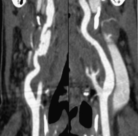
Technical advances in CTA from the last decade have allowed unprecedented imaging for a number of neurovascular applications, including evaluation for carotid artery stenosis, acute ischemic and hemorrhagic stroke, intracranial vascular anomalies, and craniocervical trauma. By far the most common indication for CTA of the extracranial circulation is for suspected carotid artery stenosis due to atherosclerosis (Fig. 14-1). Computed tomographic angiography is also part of the comprehensive evaluation of the patient with an acute stoke, where nonenhanced brain CT, vascular angiography, and perfusion imaging can be acquired during the comprehensive CT examination. Nonatherosclerotic diseases such as fibromuscular dysplasia (FMD), aneurysms or pseudoaneurysms, or dissections can also be imaged with high spatial resolution (Fig. 14-2). Additionally, CTA has a unique role in follow-up after carotid artery stenting procedures (see Fig. 14-1) instead of using MRA, which typically has significant susceptibility artifacts.

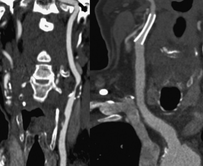
Figure 14-1 Carotid artery atherosclerosis.

Curved planar reformation (CPR) from left carotid artery shows significant stenosis and noncalcified plaque, with minor calcifications at bifurcation and hemodynamically insignificant but ulcerated plaque at common carotid artery (CCA) (left), and a widely patent right carotid artery stent (right).

(Adapted with permission from Berg M et al: CT angiography of the extracranial and intracranial circulation with imaging protocols. In Mukherjee D, Rajagopalan S, editors: CT and MR angiography of the peripheral circulation: practical approach with clinical protocols, London, 2007, Informa UK Ltd., p. 67.)

Figure 14-2 Carotid artery pseudoaneurysm.

Curved planar reformation (CPR) of right carotid artery shows large pseudoaneurysm (left) of right internal carotid, with normal-appearing left common and internal carotid arteries (right).

Diagnosis of carotid disease

MDCT has shown a 100% correlation with invasive angiography for locating significant stenosis. The interobserver agreement in evaluating total versus subtotal occlusion, stenosis length, retrograde ICA flow, and location of the stenotic site is 1.0, 0.94, 0.86, and 0.89, respectively.^24,³⁹ MDCT is also helpful in identifying underlying etiology such as dissection, atherosclerosis, or thrombosis. Berg et al. studied 35 consecutive symptomatic patients with cerebrovascular disorders (e.g., minor stroke, transient ischemic attack (TIA), amaurosis fugax, dizziness) and performed MD-CTA.²⁴ The main focus of the study was comparing MD-CTA to conventional x-ray DSA and rotational DSA as reference standards. In this study, the degree of stenosis was slightly underestimated with CTA, with mean differences (± standard deviation) per observer of 6.9 ± 17.6% and 10.7 ± 16.1% for cross-sectional, and 2.8 ± 19.2% and 9.1 ± 16.8% for oblique sagittal MPRs, compared with x-ray and rotational angiography, respectively. Computed tomographic angiography was somewhat inaccurate for measuring the absolute minimal diameter of subtotally occluded carotid arteries. For symptomatic lesions, interactive CTA interpretation combined with MPR measurements of lesions with a visual estimate of 50% or greater diameter narrowing had a sensitivity of 95% and specificity of 93% for detection of carotid stenosis compared with DSA. Based on these data, it can be concluded that CTA is sensitive for detecting significant carotid artery stenosis.

Although MD-CTA is a very effective noninvasive means of assessing cervicocranial circulation, there are multiple limitations that may occasionally restrict its usefulness. Computed tomographic angiography does not include flow dynamics. Blooming artifact due to calcification in segments can obscure the lumen and lead to overestimation of stenosis severity. Surgical clips can also preclude accurate assessment. The radiation dose of neurovascular CTA is between 1.7 and 3.0 mSv, depending on the imaged volume, type of scanner, and use of radiation reduction algorithms. There may be overlapping veins that prevent detection of small cerebral artery aneurysms.

Computed Tomographic Angiography of the Thorax

Pulmonary arteries

Technical Considerations and Clinical Applications

Pulmonary embolism (PE) is the third most common cause of cardiovascular death in the United States after ischemic heart disease and stroke, with an estimated annual incidence of 300,000 to 600,000 cases per year.⁴⁰ Even though there is a high prevalence of PE, it continues to be underdiagnosed, with only 43 to 53 patients per 100,000 being accurately identified.⁴¹

Computed tomography of the pulmonary arteries (CTPA) is the current diagnostic test of choice for assessing pulmonary thromboembolic disease. In the PIOPED-II study,⁴² CTPA was principally performed on 4-slice CT with a slice thickness of 1 to 1.25 mm. In this study, the overall positive predictive value in diagnosing PE was 86% (97% for proximal, 68% for segmental, and 25% for subsegmental thrombus), and the negative predictive value was 95%. The value of CTPA varied with the clinical pretest probability of PE: in patients with high or intermediate clinical probability, the positive predictive value for PE was 96%. However, in the face of low clinical pretest likelihood, 42% of patients had a false-positive CTPA result. Therefore, a positive CTPA that was discordant with clinical data had little diagnostic value, at least on the basis of this study. There are randomized controlled studies using later-generation CT scanners that have addressed the issue of their superiority over the 4-slice systems used in PIOPED-II.⁴³^–⁴⁵ The expectation is that thinner detectors and larger detector assembly would allow rapid imaging of the pulmonary artery and branches in a few seconds, avoiding motion artifact.

To perform CTPA, the patient is placed supine with the hands above the head. Following the topogram, the field of view is prescribed to include the adrenals to the lung apices. The goal is to acquire the study with the thinnest slice collimation with a single short breath-hold in full-suspended respiration. The voltage, current, and pitch will vary depending on vendor and patient characteristics. There are two main methods for image acquisition: timing bolus and bolus tracking techniques. In the timing bolus technique, a region of interest is placed in the pulmonary trunk, and repeated scans are acquired at the same level every 2 to 4 seconds. A time density curve is obtained, allowing for calculation of the scan delay. The alternate approach is using an automated bolus tracking technique, where a region of interest is placed over the pulmonary trunk, and the image acquisition initiates once a specified attenuation threshold is achieved. The pulmonary arteries are imaged with the first pass of IV contrast, and the pelvis and lower-extremity veins can be imaged later with a scan delay of 2.5 to 3.5 minutes.

CTPA images can be reconstructed using several techniques; however, one suggested method is using a 1.25-mm slice thickness with a 50% to 60% slice increment. Larger slice thickness is used for reconstruction of the pelvis and lower-extremity veins. There are multiple artifacts that can limit detection of true PEs, so careful scrutiny of the acquired images with active scrolling in and out of each main, lobar, segmental, and subsegmental artery is necessary to avoid overcalling or missing PEs. Similarly, CT venography of the proximal lower extremities is difficult to interpret and suffers from several technical limitations, such as flow artifacts from suboptimal timing of contrast, arterial inflow contamination, streak artifacts from orthopedic hardware, arterial calcification, or dense contrast within the bladder.

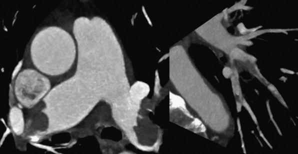
The CTPA findings of acute PE can be divided into arterial findings and ancillary findings. Intraluminal filling defects may partially or completely occlude a pulmonary artery and typically cause significant dilation of the vessel. Acute emboli appear as adherent intravascular filling defects that form acute angles to the vessel wall, whereas chronic thrombi have the appearance of mural adherent thrombi contiguous with the vessel wall. Acute PEs that straddle the bifurcation of the left and right pulmonary arteries are referred to as saddle emboli (Fig. 14-3). Lung infarcts, atelectasis, and oligemia of the affected territory are common lung parenchymal findings with a PE.