, Brian C. Healy2 and Brian C. Healy3
(1)
Department of Biostatistics, Massachusetts General Hospital, Boston, MA, USA
(2)
Harvard Medical School, Boston, USA
(3)
Harvard School of Public Health Biostatistics Center, Department of Neurology, Massachusetts General Hospital, Boston, MA, USA
Abstract
A general understanding of statistical concepts is necessary for any cardiologist intending to either perform scientific research or understand the results of others’ research. The field of statistics is often broken down into two branches: descriptive statistics and inferential statistics. This chapter provides a review of each of these branches and also gives a summary of statistical concepts related to clinical research. Our goal in this chapter is both to prepare readers to successfully answer statistics questions on the cardiology board exams and to provide readers with statistical background knowledge related to clinical trials and medical research. Readers interested in a more thorough discussion of statistical concepts should consult Bernard Rosner’s (Fundamentals of biostatistics, 7th edn. Duxbury Press, Belmont, 2010) or Rothman et al. (Modern epidemiology, 3rd edn. Lippincott Williams & Wilkins, Philadelphia, 2008).
Abbreviations
ACCORD
Action to Control Cardiovascular Risk in Diabetes
AF
Atrial fibrillation
AHA
American Heart Association
ANOVA
Analysis of variance
AUC
Area under the curve
BNP
Brain natriuretic peptide
CABG
Coronary artery bypass graft
CHF
Congestive heart failure
CI
Confidence interval
CVD
Cardiovascular disease
ECG
Electrocardiogram
ER
Emergency room
FN
False negatives
FP
False positives
H0
Null hypothesis
H1
Alternative hypothesis
HR
Hazard ratio
IQR
Interquartile range
LR+
Positive likelihood ratio
LR−
Negative likelihood ratio
MI
Myocardial infarction
NPV
Negative predictive value
NT-proBNP
N-terminal prohormone of brain natriuretic peptide
NYHA
New York Heart Association
OR
Odds ratio
PPV
Positive predictive value
PRIDE
Pro-BNP Investigation of Dyspnea in the Emergency Department
ROC
Receiver operating characteristic
SD
Standard deviation
SOC
Standard of care
TN
True negatives
TP
True positives
Introduction
A general understanding of statistical concepts is necessary for any cardiologist intending to either perform scientific research or understand the results of others’ research. The field of statistics is often broken down into two branches: descriptive statistics and inferential statistics. This chapter provides a review of each of these branches and also gives a summary of statistical concepts related to clinical research. Our goal in this chapter is both to prepare readers to successfully answer statistics questions on the cardiology board exams and to provide readers with statistical background knowledge related to clinical trials and medical research. Readers interested in a more thorough discussion of statistical concepts should consult Bernard Rosner’s [1] or Rothman et al. [2].
Descriptive Statistics
Goal of Descriptive Statistics
To describe the characteristics of a sample of data. Example—baseline characteristics of a study sample.
Types of Data
Categorical (also known as nominal): A variable that can take on two or more values, but there is no ordering of the values. Examples—race, occupation, marital status.
Dichotomous (also known as binary): A categorical variable that can take on only two values. Examples—normal/abnormal, yes/no, dead/alive.
Ordinal (also known as rank): A variable that can take on two or more categories with a clear ordering but not necessarily equal magnitude between categories. Examples—NYHA grade, mild/moderate/severe.
Continuous: A variable that can take on an entire range of values with a clear ordering and magnitude of difference. Examples—age, lab values, expression levels.
Time-to-event: A variable that measures the amount of time between two events, typically including censored observations (that is, observations for which only partial information is available). Example—time to death (patients who were alive at the date of last contact are censored since the death/event had not occurred).
Summary Statistics
Dichotomous, Categorical :
Frequency: n, the number of sample members within each category.
Proportion: , the percent of sample members within each category, where n is the frequency of the category and N is the total sample size.
Continuous :
Sample mean: , the most commonly used measure of location, but can be affected by outliers or skewed distribution. This is equal to the sum of the observations divided by the number of observations.
Sample standard deviation (SD): , the most commonly used measure of variability, but can be affected by outliers or skewed distribution.
Sample median: The 50th percentile (i.e. the value that is both >50 % of the sample and <50 % of the sample). This is the most appropriate measure of location for skewed data. For normally distributed data, the median equals the mean.
Sample interquartile range (IQR): The difference between the 75th percentile and the 25th percentile, typically reported with the median for skewed distribution.
Incidence and Prevalence:
Prevalence: The proportion of the population with a disease or condition of interest.
Incidence rate: The rate of new cases in a given time frame.
Example—
Inferential Statistics
Goal of Inferential Statistics
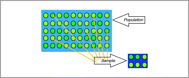
To use a sample (Fig. 13-1) to draw conclusions about a population.


Figure 13-1
Selecting a random sample from a population
Outcome variable: The dependent variable or the variable to be predicted in an experiment.
Explanatory variable(s): The independent variable(s) or the variable(s) used to predict the outcome variable.
Estimation
A common goal in medical research is to estimate a quantity of interest.
Point estimate: To estimate a population parameter, we use the sample estimate based upon the type of data (described above). Examples–We can use the sample mean to estimate the population mean, or we can use the sample proportion of success to estimate the population probability of success.
Interval estimate/Confidence intervals (CI): Gives a range of plausible values for the estimate. In other words, gives a sense of the variability of a sample estimate. Formally, a 95 % CI says if you resample a population 100 times, you expect on average 95 of the CIs to cover the true population parameter and 5 of the CIs to not cover the true population parameter.
Example: Ho et al. [3] reported that the Framingham age-adjusted hazard ratio (HR) of death (95 % CI) following congestive heart failure for women vs men was 0.64 (0.54, 0.77). This means that our best guess of the true population hazard ratio is 0.64, but any value from 0.54 to 0.77 is considered plausible based on this study.
Hypothesis Testing
A second common goal in medical research is to compare a quantity of interest to a known value or to compare a quantity of interest in two (or more) groups using a hypothesis test.
Reasons for differences between groups:
Actual effect—Observed difference occurred because there truly is a difference between groups.
Chance—Observed difference occurred due to random differences among samples drawn from the population. Statistical tests are designed to determine if observed differences were likely due to chance.
Bias—Observed difference occurred because of intentional or unintentional errors in the study design.
Confounding—Observed difference was caused by another factor that was associated with the groups.
Hypothesis testing :
A formal statistical procedure to assess if the observed result is unlikely due to chance under the null hypothesis.
Null hypothesis (H 0 )/Alternative hypothesis (H 1 ): Two statements about the relationship between groups that cover all possibilities. Our goal is to make a statement about H0 (either reject or fail to reject H0) based on the available data. H0 is often set up so that there is no difference between groups so that we can reject the null in favor of a difference.
One-sided hypothesis test: A hypothesis test in which the alternative of interest is in only one direction. Example – H0: Mean cholesterol in treated patients is higher than or equal to the mean cholesterol in placebo treated patients; H1: Mean cholesterol in treated patients is lower than the mean cholesterol in placebo treated patients
Two-sided significance test: A hypothesis test in which the alternative of interest is in both directions. This is a more conservative test and is more commonly reported in the literature. Example – H0: Mean cholesterol in males is equal to the mean cholesterol in females; H1: Mean cholesterol in males is not equal to the mean cholesterol in females
Errors
Type I error: Rejecting a null hypothesis when the null hypothesis is actually true (false positive).
Type II error: Failing to reject the null hypothesis when the null hypothesis is actually not true (false negative).
Significance level: The probability of a type I error, also called the alpha-level, usually set to 0.05. This is how often we allow a type I error if we test the hypothesis at this level.
p-value: The probability of obtaining the observed result or something more extreme assuming that the null hypothesis is true. If the p-value is less than the significance level, we reject the null hypothesis.Parametric vs. non-parametric test
Parametric test: A hypothesis test that assumes the data being analyzed come from a specific distribution (e.g., normally distributed). When these assumptions are met, these tests tend to increase statistical power.
Non-parametric test: A hypothesis test that makes fewer assumptions about the distribution of the data but often has less statistical power.
Steps for Hypothesis Testing
1.
Experimental question
(a)
State your null and alternative hypotheses.
(b)
State the type of data for the outcome and explanatory variable(s).
(c)
Determine the appropriate statistical test.
2.
Computation
(a)
State the appropriate summary statistic.
(b)
Calculate the p-value.
3.
Interpretation
(a)
Decide whether to reject or not reject the null hypothesis.
(b)
State your conclusion.
Statistical Tests
Statistical tests to be used for given outcome and explanatory variable types are shown in Table 13-1. For a more complete list, see http://www.ats.ucla.edu/stat/mult_pkg/whatstat/default.htm.
Table 13-1
Statistical tests to be used for given outcome and explanatory variable types
Outcome Variable | Explanatory Variable | Statistical Test | Effect estimate | |
|---|---|---|---|---|
Continuous | Dichotomous | t-test, Wilcoxon test, linear regression | Difference in group means | |
Continuous | Categorical | ANOVA, linear regression | Difference in group means | |
Continuous | Continuous | Correlation, linear regression | Correlation coefficient | |
Dichotomous | Dichotomous | Chi-squared test (Fisher’s exact test), logistic regression | Odds ratio | |
Dichotomous | Categorical | Chi-squared test, logistic regression | Odds ratio | |
Dichotomous | Continuous | Logistic regression | Odds ratio | |
Time-to-event | Dichotomous | Log-rank, Cox regression | Hazard ratio | |
Time-to-event < div class='tao-gold-member'>
Only gold members can continue reading. Log In or Register to continue
Stay updated, free articles. Join our Telegram channel
Full access? Get Clinical Tree
 Get Clinical Tree app for offline access

|