Regulatory agencies, professional societies, and clinical trialists commonly base judgments of treatment benefit on separate assessments of efficacy and safety. When separate assessments were compared with an integrated assessment using a kinetic model of a hypothetical randomized trial of antiplatelet agents in patients with acute coronary syndrome, the former showed treatment A to be superior to treatment B, whereas the latter showed treatment B to be superior to treatment A. In conclusion, comparative judgments regarding the balance between efficacy and safety depend on the model chosen for analysis; kinetic models are particularly suited to the integrated assessment of efficacy and safety relative to regulatory decisions, public policy, guideline development, and clinical care.
How complicated and unpredictable the machinery of life really is.
The US Food and Drug Administration requires formal quantitative demonstrations of efficacy and safety for approval of new drugs and devices for marketing. Professional guideline committees such as those sponsored by the American College of Cardiology and the American Heart Association, however, rely on less formal assessments of the balance between benefit and harm, whereas clinical trialists tend to assess the balance more through informal rhetorical argument than quantitative scientific exposition.
It is not surprising, then, that conflicts between efficacy and safety are frequently encountered in the assessment of drugs and devices. Thus, statins provide unquestioned benefit in terms of reduction in cardiovascular events but have been reported to increase the incidence of diabetes. Drug-eluting stents clearly reduce the need for target vessel revascularization compared with bare metal stents (a common outcome of arguable clinical importance) but are also associated with late stent thrombosis (an uncommon outcome of unquestioned clinical importance).
Balancing such trade-offs between efficacy and safety is a complex task that poses a major challenge to regulatory authorities and clinical practitioners alike. Although a number of approaches to the quantitative assessment of efficacy and safety have been advanced, they all tend to be of limited accessibility to practitioners. The purpose of this perspective, then, is to propose a more accessible approach to the integrated assessment of efficacy and safety.
HASEY: Hypothetical Assessment of Efficacy and Safety
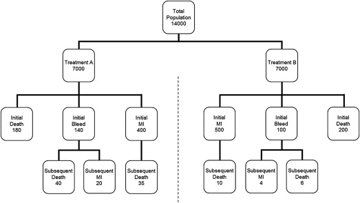
Consider a fictitious clinical trial called HASEY (Hypothetical Assessment of Safety and EfficacY) in which 14,000 patients are randomized to 2 different platelet inhibitors (treatment A or treatment B) and followed for 15 months. The primary efficacy end point is a composite comprising the first occurrence of death or nonfatal myocardial infarction (MI), whereas the primary safety end point is represented by nonfatal bleeding. This fictitious trial is roughly similar to a prototypical trial comparing prasugrel and clopidogrel in patients with acute coronary syndrome. The baseline analysis of safety and efficacy in our fictitious trial is directly analogous to that performed in the prototypical trial.
Baseline analysis
Putative outcomes for HASEY are summarized in Figure 1 and Table 1 . The composite efficacy end point occurred in 580 of 7,000 patients (8.3%) randomized to treatment A versus 700 of 7,000 patients (10.0%) randomized to treatment B (relative risk 0.83, 95% confidence interval [CI] 0.75 to 0.92, p <0.001). Efficacy was therefore significantly better with treatment A. In contrast, bleeding occurred in 140 patients (2.0%) randomized to treatment A versus 100 patients (1.4%) randomized to treatment B (relative risk 1.40, 95% CI 1.09 to 1.81, p = 0.01). Safety was therefore significantly better with treatment B. Accordingly, the practical relevance of this trial (to clinicians and regulators) depends on a clear-cut characterization of the hazy trade-off between these competing outcomes. Simply stated, does the benefit outweigh the harm?
| Outcome | Treatment A n | Treatment B n | RR | 95% CI | p |
|---|---|---|---|---|---|
| Initial death | 180 | 200 | 0.90 | 0.74–1.10 | 0.299 |
| Initial MI | 400 | 500 | 0.80 | 0.70–0.91 | 0.001 |
| Composite benefit | 580 | 700 | 0.83 | 0.75–0.92 | <0.001 |
| Initial bleed | 140 | 100 | 1.40 | 1.09–1.81 | 0.010 |
| Net benefit | 720 | 800 | 0.90 | 0.82–0.99 | 0.030 |
To their credit, the HASEY investigators anticipated there would be a trade-off between safety and efficacy associated with platelet inhibition, and therefore prespecified a “net benefit” end point represented by the simple sum of the individual component outcomes. As listed in Table 1 , a total of 720 of these events (10.3%) were associated with treatment A versus 800 of these events (11.4%) associated with treatment B (relative risk 0.90, 95% CI 0.82 to 0.99, p = 0.03). Based on this analysis, the investigators concluded that the benefit of treatment A outweighs its harm.
Unfortunately, this analysis relies only on the first occurrence of the component events and, therefore, ignores all the subsequent events (e.g., death after an initial MI). As it happens, we can perform a supplementary analysis to address this limitation. According to the bottom row in Figure 1 , there were 95 subsequent events in the patients assigned to treatment A and 20 subsequent events in the patients assigned to treatment B. If we ignore the influence of double counting, add the subsequent events to the initial events, and then analyze the total, as some investigators recommend, the difference in “net benefit” between treatment A and treatment B becomes statistically nonsignificant (relative risk 0.99, 95% CI 0.91 to 1.09, p = 0.90). Of course, any such analysis can change markedly based on the specific distribution of the component outcomes in the initial and final tallies, and the magnitude of this change would need to be explored through sensitivity analyses over realistic ranges of outcome events. Even so, this seems a rather ad hoc way to characterize potentially important differences between efficacy and safety, especially because it fails to consider the individual component end points as competing risks relative to efficacy and safety.
Cox regression analysis
An alternative way to address this issue would be to perform a Cox proportional hazards regression on the patient level time-to-event data. Accordingly, hypothetical patient level time-to-event data (right censored at 15 months) were generated from the population level data in Table 1 on the assumption that time-to-event is exponentially distributed as a typical Poisson process, in which events occur continuously and independently at a constant average rate. Cox regressions were performed on these hypothetical patient level data relative to each of the end points in Table 1 using WinSTAT (version 2012.1) (R. Fitch Software, www.winstat.com ). The resultant hazard ratios listed in Table 2 were essentially identical to the risk ratios in Table 1 .
| Outcome | Treatment A n | Treatment B n | HR | 95% CI | p |
|---|---|---|---|---|---|
| Initial death | 178 | 200 | 0.89 | 0.73–1.09 | 0.251 |
| Initial MI | 405 | 506 | 0.79 | 0.70–0.91 | <0.001 |
| Composite benefit | 583 | 706 | 0.81 | 0.73–0.91 | <0.001 |
| Initial bleed | 139 | 100 | 1.39 | 1.08–1.80 | 0.012 |
| Net benefit | 722 | 806 | 0.89 | 0.80–0.98 | 0.020 |
An additional analysis relative to nonfatal MI, which incorporated bleeding and death as competing covariate risks, confirmed the superiority of treatment A over treatment B (hazard ratio 0.79, 95% CI 0.70 to 0.91, p = 0.001). This analysis, however, did not identify bleeding or death to have an independent association with treatment benefit (hazard ratio 1.04, 95% CI 0.64 to 1.71, p = 0.86 for bleeding and hazard ratio 1.37, 95% CI 0.98 to 1.97, p = 0.06 for death). Thus, judgments regarding the balance between efficacy and safety clearly depend on the model used in the analyses.
Kinetic analysis
Kinetic modeling might provide a more transparent, internally consistent way to integrate the assessment of efficacy and safety. Such models have been used for centuries in the physical sciences, and have been successfully applied to the study of a variety of biologic processes.
Briefly, a kinetic model quantifies the time-dependent transition from state A to state B (denoted A→B), the states being expressed in terms of binomial proportions (denoted [A] and [B]), and the time dependence being expressed in terms of a constant of proportionality or rate constant (k). The canonical transition of this kind is that of a monotonic exponential decay ([A] = e −kt ), where [A] = 1 at t = 0, the rate of change for [A] is inversely proportional to its presence, and the constant of proportionality, k, is the hazard (in units t −1 ):
ⅆ [ A ] ⅆ t = − k [ A ]
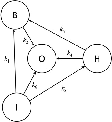
Assuming that each of the multiple state-to-state transitions leading to an event obeys this simple exponential law (equivalent to the proportional hazards assumption in Cox regression), we can construct a plausible kinetic model of any clinical trial in terms of the network of transitions and rate constants derived from its empirical observations ( Figure 2 ). With respect to HASEY, then, the initial state I is characterized by the pretreatment inclusion and/or exclusion criteria that are operative at the time of randomization, the intermediate state B is the end point indicative of treatment benefit (nonfatal MI), the intermediate state H is the end point indicative of treatment harm (nonfatal bleeding), and the terminal outcome state O, common to both, is represented by death. Although each of these transitions is theoretically reversible (even death can be reversed by cardiopulmonary resuscitation), no such events appear in Figure 1 . Were reversible transitions to occur, however, the model is readily modified to represent them.
As summarized in the Appendix , we can express this model in terms of a simultaneous set of ordinary differential equations (hazard functions) representing each of the state transitions in Figure 2 . The proportion of each state over time is therefore defined by the rate equations derived through mathematical integration of these hazard functions. According to these rate equations, efficacy and safety are thereby shown to be complex interrelated functions of these proportions and their rates of change.
The empirical rate constants, along with their associated standard errors, were evaluated from the data in Figure 1 using conventional statistical techniques ( Table 3 ). Statistical significance of an observed change was defined by a 2-sided p value <0.05. Clinical importance of the change in hazard ratio was defined by Bayesian analysis as a relative difference in excess of 10% (<0.9 or >1.1), using a moderately skeptical prior for which the probability is under 5% that the difference is >25%. For each treatment, the time course of each outcome was defined through a global sensitivity analysis of the cumulative standard errors for the kinetic rate equations using simultaneous bootstrap resampling of the aggregate set of log-normally distributed rate constants (1,000 runs for each).
| State | Treatment A N = 7000 | Treatment B N = 7000 | ||||||
|---|---|---|---|---|---|---|---|---|
| n | p ± σ | t | k ± σ | n | p ± σ | t | k ± σ | |
| I→B | 400 | 0.057 ± 0.003 | 14.6 | 0.0040 ± 0.0002 | 500 | 0.071 ± 0.003 | 14.5 | 0.0051 ± 0.0002 |
| B→O | 35 | 0.088 ± 0.014 | 7.2 | 0.0128 ± 0.0022 | 10 | 0.020 ± 0.006 | 7.4 | 0.0027 ± 0.0009 |
| I→H | 140 | 0.020 ± 0.002 | 14.9 | 0.0014 ± 0.0001 | 100 | 0.014 ± 0.001 | 14.9 | 0.0010 ± 0.0001 |
| H→O | 40 | 0.286 ± 0.038 | 6.4 | 0.0523 ± 0.0083 | 6 | 0.060 ± 0.024 | 7.3 | 0.0085 ± 0.0035 |
| H→B | 20 | 0.143 ± 0.030 | 7.0 | 0.0221 ± 0.0050 | 4 | 0.040 ± 0.020 | 7.4 | 0.0056 ± 0.0028 |
| I→O | 180 | 0.026 ± 0.002 | 14.8 | 0.0018 ± 0.0001 | 200 | 0.029 ± 0.002 | 14.8 | 0.0020 ± 0.0001 |
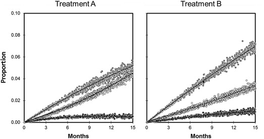
The proportion of each component end point during the 15-month duration of the trial based on the sensitivity analysis of the kinetic parameters in Table 3 is illustrated in Figure 3 . Comparisons between treatment A and treatment B after 15 months of follow-up are summarized in Table 4 and Table 5 , in contrast to those for the baseline analysis summarized in Table 1 . Based on these data, treatment A is associated with a lower proportion of nonfatal MI and bleeding, but a greater proportion of death. All these differences are statistically significant and of a magnitude deemed to be clinically important at the operative 10% threshold.
| Transition | HR | 95% CI | p | P HR<0.9 | P HR>1.1 |
|---|---|---|---|---|---|
| I→B | 0.79 | 0.69–0.90 | <0.001 | 0.976 | <0.001 |
| B→O | 4.69 | 2.32–9.48 | <0.001 | <0.001 | >0.999 |
| I→H | 1.41 | 1.09–1.82 | 0.009 | <0.001 | 0.970 |
| H→O | 6.15 | 2.61–14.52 | <0.001 | <0.001 | >0.999 |
| H→B | 3.99 | 1.36–11.66 | 0.012 | 0.003 | 0.991 |
| I→O | 0.90 | 0.73–1.10 | 0.292 | 0.511 | 0.024 |
| Endpoint | Treatment A p ± σ | Treatment B p ± σ | RR | 95% CI | p | P RR<0.9 | P RR>1.1 |
|---|---|---|---|---|---|---|---|
| [B] | 0.052 ± 0.003 | 0.072 ± 0.003 | 0.72 | 0.63–0.83 | <0.001 | 0.999 | <0.001 |
| [H] | 0.007 ± 0.001 | 0.012 ± 0.001 | 0.57 | 0.47–0.69 | <0.001 | >0.999 | <0.001 |
| [O] | 0.043 ± 0.003 | 0.031 ± 0.002 | 1.43 | 1.18–1.73 | <0.001 | <0.001 | 0.996 |
Comparison of the baseline and kinetic analyses
At first blush, these findings may seem paradoxical. The intermediate proxies for efficacy and safety are better with treatment A, whereas, “net benefit” in terms of subsequent mortality is better with treatment B. Analysis of the individual rate constants, however, serves to explain this apparent paradox. Recall that the baseline comparisons summarized in Table 1 demonstrated that treatment A was associated with a risk ratio of 0.80 for initial MI and a risk ratio of 1.40 for initial bleeding. This is consistent with the kinetic analysis in Table 4 which demonstrates that treatment A is associated with a hazard ratio of 0.79 for the transition I→B and a hazard ratio of 1.41 for the transition I→H (in agreement with the supplemental Cox regressions). According to Table 4 , however, the hazard ratios for the subsequent transitions are much greater (4.69 for B→O and 6.15 for H→O). Consequently, the intermediate states (MI and bleeding) disappear more quickly than they appear. As a result, the observed proportions of these states are less than expected and the observed proportion of the terminal state (total mortality) is more than expected. Treatment A is therefore superior to treatment B with respect to the intermediate outcomes but inferior to treatment B with respect to the terminal outcome ( Figure 3 ). The baseline analysis summarized in Table 1 is blind to these nuanced distinctions.
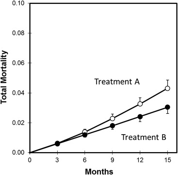
Because death is the common terminus for both benefit and harm in this model, a direct comparison of treatment A versus treatment B with respect to total mortality serves as an overall index of the balance between efficacy and safety ( Figure 4 ). According to this assessment, treatment A is thereby adjudged inferior to treatment B (relative risk 1.43, 95% CI 1.18 to 1.73, p <0.001, P RR>1.1 = 0.996). This is very different from the baseline assessment summarized in Table 1 , according to which treatment A was adjudged superior to treatment B (relative risk 0.90, 95% CI 0.82 to 0.99, p = 0.03). Although these differences do not directly challenge the conclusions of the prototypical trial on which this pedagogical exercise is founded, they nonetheless underscore the importance of subjecting such trials to a robust range of alternative analyses.
In this context, a recent study compared the performance of alternative stochastic models for analysis of repeated ischemic events among all components of the primary end point (all cause death, MI, or stroke) in the Targeted Platelet Inhibition to Clarify the Optimal Strategy to Medically Manage Acute Coronary Syndromes (TRILOGY ACS) trial. The investigators concluded that models accounting for all events, especially those incorporating subjective weightings indicative of the clinical relevance of the individual components appeared most advantageous.
Clinical and Regulatory Considerations
So which of these alternatives are we to believe—the prototypical analysis based on the unfounded assumption that each of the component outcomes is equal in importance or the kinetic analysis based on the actual pattern of empirical observations?
Just as we cannot combine different physical weights unless they are expressed in the same units of mass (kilograms vs pounds), we cannot combine different clinical outcomes (death vs nonfatal MI) unless they too are expressed in the same units of importance. However, how do we come up with a suitable conversion factor? How many nonfatal MIs are equal in importance to 1 death?
There is more than a single answer this question. Metrics such as “number-needed-to-treat” (NNT) and “number-needed-to-harm” (NNH) or their ratio (NNT/NNH) are sometimes used as conversion factors to assess the balance between efficacy and safety. According to the usual interpretation of these metrics, treatment is warranted if NNT < NNH or if NNT/NNH <1. However, although NNT and NNH are relatively simple to compute (being the reciprocals of the absolute differences in risk) and generally familiar to physicians, their use assumes that the operative measures of benefit and harm have equivalent clinical importance. One way to deal with this limitation is through decision analysis, by which each of these measures is adjusted in terms of its expected value (the summed product of the individual utilities and their probabilities) or relative utility (the utility associated with an instance of benefit vs the [dis]utility associated with an instance of harm). An alternative approach, similar to that used in cost-effectiveness analyses, is to adjust the difference between the measures by some index of proportionality (the observed benefit minus the observed harm divided by a factor representing the maximum instance of harm one is willing to tolerate for each instance of benefit). It goes without saying that all such adjustments are decidedly subjective.
A more objective approach might be based on the case-fatality rates of the component outcomes internal to the trial—the probability of subsequent death after an initially nonfatal outcome during the duration of follow-up. For example, there were 924 cases of MI in our hypothetical trial, 45 of which were fatal—a case-fatality rate of 4.9 ± 0.7%. Similarly, there were 240 episodes of bleeding, 46 of which were fatal—a case-fatality rate of 19.2 ± 2.5%. These rates allow us to convert the number of nonfatal outcomes for each component into an “effective” number of fatal outcomes, which can then be added to the actual number of fatal outcomes. Based on this accounting, there are 293 effective fatalities associated with treatment A versus 258 of those associated with treatment B. According to this analysis, treatment A would be adjudged slightly, but not importantly, inferior to treatment B (relative risk 1.14, 95% CI 0.96 to 1.34, p = 0.13, P RR>1.1 = 0.648).
The principal limitation of case-fatality rates, however, is the assumption that they encapsulate all the important effects of a drug or device relative to efficacy and safety. This is clearly not the case. Some nonfatal outcomes very likely have important clinical, economic, and social consequences that will be obscured by the use of case-fatality rates. If a treatment causes an important degree of nonfatal infirmity, for example, this will have little influence on the weighting relative to safety despite having a substantial influence on quality of life. Reducing a clinical trial to a simple assessment of “effective mortality”, therefore, may oversimplify its interpretation.
Kinetic models, as a feature of their design, mitigate these difficulties by disentangling the complex interactions between fatal and nonfatal outcomes. Thus, if a treatment has a direct effect on mortality, this will manifest itself as a change in the rate constants representative of the terminal transitions (I→O, B→O, H→O). In contrast, if the treatment has an indirect effect on mortality, this will manifest itself as a change in the rate constants for the intermediate transitions representative of efficacy (I→B) and safety (I→H). The range of alternatives is substantial. Because our hypothetical trial comprises 6 independent transitions, each with 3 patterns of response (the rate constant can increase, decrease, or remain unchanged), there are 3 6 or 729 possibilities (3 12 or 531,441 possibilities if all 6 transitions are reversible) compared with only 2 possibilities for a simple dichotomous assessment of “net benefit”. Some of these patterns might describe surprising “black swans” such as ILLUMINATE (Investigation of Lipid Level Management to Understand its Impact in Atherosclerotic Events) in which a therapeutic increase in high density lipoprotein cholesterol was associated with a counterintuitive increase in cardiovascular events and CAST (Cardiac Arrhythmia Suppression Trial) in which therapeutic inhibition of ventricular ectopy was associated with an unanticipated increase in cardiac death. Other patterns might describe the competitive risks associated with some composite outcomes.
Kinetic models of efficacy and safety possess a number of distinct advantages that justify their added mathematical complexity. They are empirically grounded and highly flexible in design; broadly applicable to a wide range of drug and device assessments; and directly facilitate open communication among academic trialists, industry sponsors, regulatory analysts, and clinical practitioners regarding the values and judgments that impact on their decisions. Such assessments have important implications not only for clinical care but also for guideline development and regulatory policy. This is especially important when efficacy and safety are measured on different scales of clinical utility or over differing durations of follow-up.
Beyond its mathematical complexity, the key limitation of this kinetic model relates to the assumption regarding the proportionality of the hazards. This assumption is readily verified, however, by documenting the linearity of the relation between the logarithm of the empirical proportion of the outcome and follow-up time (in which the slope of the regression line is the rate constant).
Nevertheless, there are important practical limits to the assessment of safety and efficacy. Safety, even if demonstrated in the near term, can always be undermined by longer term experience. It might take years, for instance, to uncover the cancer risk associated with a new drug. Formal demonstrations of efficacy, in contrast, are more likely to stand the test of time but they too can be unreliable. Thus, investigators were able to reproduce the results in only 6 of 53 “landmark” cancer studies published in high-impact scientific journals. Not surprisingly, then, the ultimate practical utility of new drugs and devices is usually identified, not by industry sponsors or federal regulators but by practicing clinicians treating large numbers of patients over the years once these products make it to market. Thus, although the needs of patients, physicians, and health-care regulators will not always coincide, it is clearly in the best interests of all to champion practical and transparent ways to integrate judgments of safety and efficacy as the basis for clinical care and health policy. Pending its comparison with more conventional alternatives, kinetic modeling seems particularly suited to this task.
Disclosures
The author has no conflicts of interest to disclose.
Appendix
Each of the transitions in Figure 2 can be represented as a first order process (equivalent to a monotonic exponential decay), where [A] = 1 at t = 0, the rate of change for [A] is inversely proportional to its presence, and a rate constant, k, is the hazard:
Integration and rearrangement of this equation with respect to t allows k to be evaluated in terms of the observed proportion of the outcome state over the duration of follow-up:
A kinetic model for the network of transitions in Figure 2 is thereby defined in terms of the following set of ordinary differential equations (hazard functions):
ⅆ [ I ] ⅆ t = − ( k 1 + k 3 + k 6 ) [ I ] ⅆ [ B ] ⅆ t = k 1 [ I ] − k 2 [ B ] + k 5 [ H ] ⅆ [ H ] ⅆ t = k 3 [ I ] − ( k 4 + k 5 ) [ H ] ⅆ [ O ] ⅆ t = k 2 [ B ] + k 4 [ H ] + k 6 [ I ]
Stay updated, free articles. Join our Telegram channel

Full access? Get Clinical Tree


