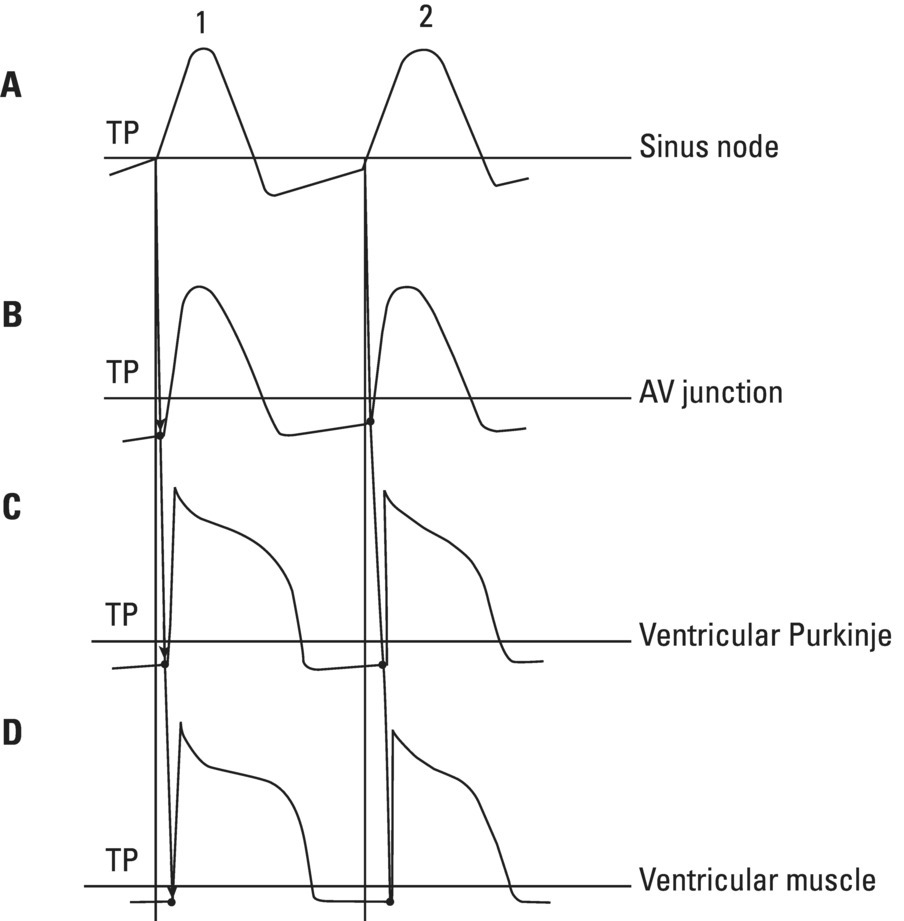
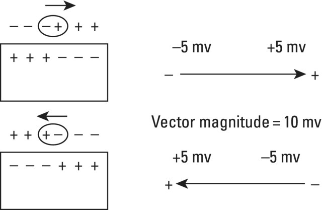
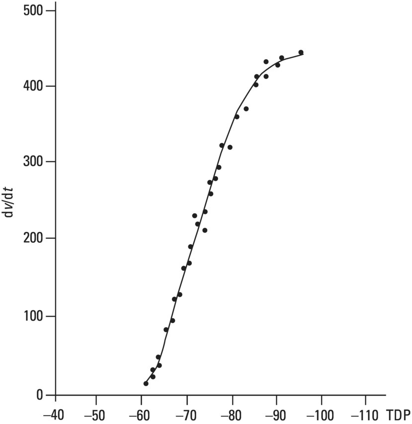
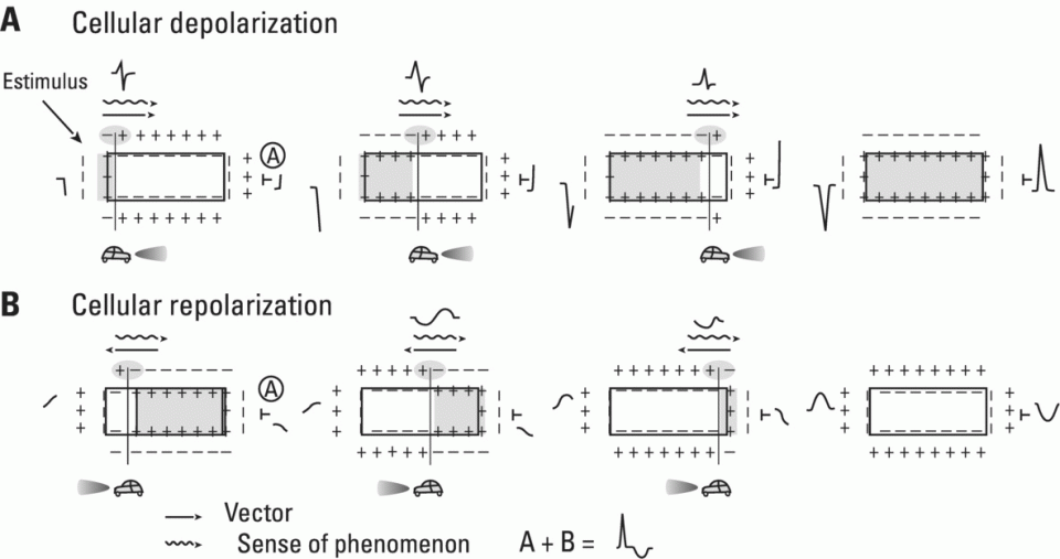
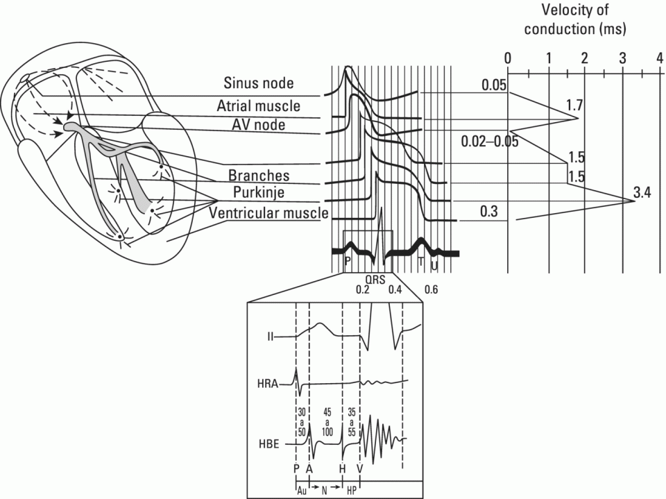
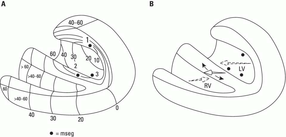
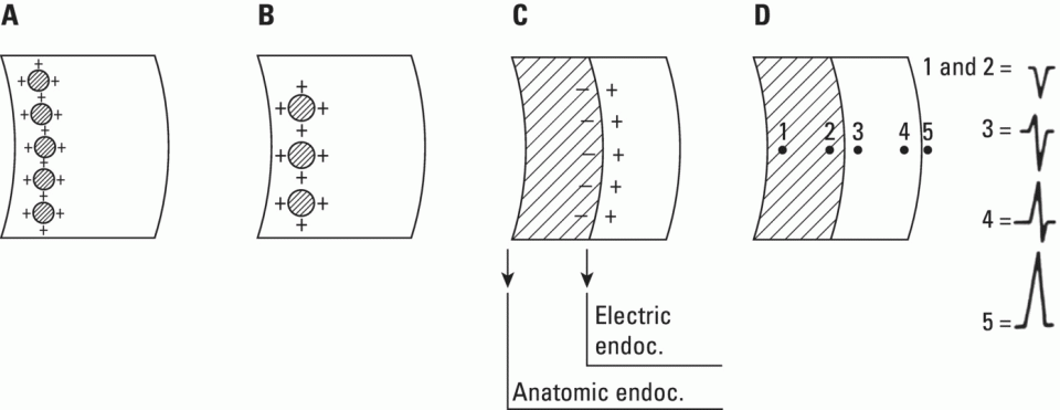
From an electrophysiological point of view, the cardiac cells previously discussed may be grouped into two different categories (Figures 5.1 and 5.2): (i) automatic slow response cells (the sinus node P cells and, to a lesser extent, some of the atrioventricular (AV) junction cells) and (ii) fast response cells (contractile cells being the prototype of these cells). Purkinje cells are considered fast response cells, but they also have some automatic potential (Figure 5.2). Transitional cells, as the name suggests, display an intermediate transmembrane action potential (AP) between the contractile cells, the Purkinje cells, and the P cells. The electrophysiological characteristics during the diastole, or resting phase (transmembrane diastolic potential (DP)), and the systole, or activation phase (depolarization plus repolarization–AP) of each cell type are different. This explains why one type of cell has an automatic behavior while the other type does not. Figures 5.1–5.3 show the different characteristics of fast and slow response cells. A distinctive characteristic of these cells is how they recover excitability; in rapid response cells, recovery is voltage‐dependent, while in slow response cells, recovery is time‐dependent. Contractile cells are polarized during the diastolic phase. This means that there is a balance between the positive charges outside the cell (Na+, Ca2+, and, to a lesser extent, K+) and the negative charges inside the cell, mainly, the non‐diffusible anion negative charges [A−], which outnumber the K+ ion, the most important positive intracellular ion (Figure 5.4A). When two separate microelectrodes are placed on the external surface of a contractile cell in the resting phase, a horizontal line is recorded (baseline line at zero level), suggesting that there is no potential difference on the cell surface. However, if an electrode is placed inside the cell, the recording will shift downward (Figure 5.4B), showing the potential difference between the outside (+) and the inside (−) of the cell. In contractile cells, this line, called the TDP, is stable (rectilinear phase 4) at −90 mV (Figures 5.1–5.4). Contractile cells show an equilibrium between inward diastolic currents of Na+Ca2+ (Ibi) and an outward K+ current (IK2). This explains why DP is not modified and remains stable. Here, DP does not reach the threshold potential (TP) (≈−70 mV) by itself, but requires the impulse to be delivered by a neighboring cell (Figure 5.5). The automatic cells of the SCS have a DP (phase 4) with an initial value of −70 mV. In this case, the inward diastolic current of Na and Ca (If) remains stable and rapidly inactivates the outward current of K (Ip) (Figure 5.2C). This initiates an ascending slope line, which rises to reach the TP by itself (≈−55 mV). Therefore, the downward K+ conductance (gK) and the upward Na+ and Ca2+ conductances (gNaCa) cross over, initiating the automatic formation of the AP (Figures 5.1–5.3). The transmembrane action potential (AP) was first recorded in 1951 by Weidman and Draper, and has four phases: phase 0, depolarization, and phases 1, 2, and 3, repolarization. We will first discuss the concept of a dipole. The term “dipole” is applied to a pair of electrical charges, (+−) or (−+), that separate a positively charged zone of the cell surface from a negatively charged zone. This pair of charges exists during depolarization and repolarization, but not when these processes are completed. An electrocardiogram (ECG) records differences in potential between the positive and negative zones. These differences in potential can be expressed using a vector departing from the negative charge and heading toward the positive charge. In this way, a vector shows a magnitude calculated using the differences of potential between the head of the vector (+) and the tail (−) (Figure 5.6). The vector is recorded as a positive or negative deflection according to whether the exploratory electrode faces the head or tail of it regardless of whether the phenomenon Figure 5.1 Transmembrane diastolic or resting potential (DP) and transmembrane action potential (AP) of contractile (A) and automatic (B) cells. Of particular note is the difference with regard to the DPs, which are rectilinear and far from zero in contractile cells and ascending and closer to zero in automatic cells. Only when the stimulus reaches the threshold potential (TP), after it is excited by a neighboring cell (a in A) or because it features an automatic capacity (B), is a AP generated. Note how in the rapid response cells (with no automatic capacity), a stimulus not reaching the TP (b and c in A) does not generate a AP (see box in A). The onset of phase 0 occurs both in automatic and contractile cells when the intersection of conductances (gK, gNaCa) (Figure 5.3) occurs at the TP level. This level in automatic cells is lower than in contractile cells (about −55 mV vs. −70 mV) (Figures 5.1 and 5.3). In the fast response cells—contractile cells—the DP is −90 mV and is stable because during diastole there is an equilibrium between the inward NaCa currents (Ibi) and the outward K currents (IK2) (Figure 5.2A). To analyze ionic changes at different levels, the voltage clamp technique is used (Coraboeuf 1971). When the DP receives a propagated impulse with sufficient strength to reach the TP, a AP is initiated. The AP in these cells is abrupt in the initial phase (start of phase 0) because the DP is far from zero (−90 mV). According to what we already know about the membrane response curve, the AP ascending velocity is greater when the DP is far from zero (Figures 5.1 and 5.7). Figure 5.2 Ionic current passing through the cellular membrane (CM) in a contractile cell (fast response cell) (A), Purkinje cell (B), and automatic cell (slow response cell) (C) during systole and diastole. During diastole, the IK2 current is constant in contractile cells (A), but not in Purkinje cells (B) (represented by a reduction of the arrow thickness in the IK2 current). The outward K current (Ip) in automatic cells is even more rapidly inactivated by the inward If current (greater reduction or even disappearance, broken arrows representing the Ip current (C)). In a fast response cell (contractile cell) (A), the DP is stable during diastole, and the NaCa current (Ibi) does not predominate over the K current. This explains why in this case Ibi and IK2 arrows generally have the same size. The ionic currents of automatic and contractile cells during systole seen in more detail in Figure 5.3. Figure 5.3 The most relevant ionic currents in automatic (A) and contractile (B) cells during systole. Contractile cells are characterized by an early and abrupt Na+ inward flow and an initial and transient K+ outward flow (Ito). These are not present in automatic cells. Figure 5.4 (A) The predominant negative charges inside the cell are due to the presence of significant non‐diffusible anions which outweigh the ions with a positive charge, especially K+. (B) Two microelectrodes placed at the surface of a myocardial fiber record a horizontal reference line during the resting phase (zero line), signifying no potential differences on the cellular surface. When one of the two electrodes is introduced inside the cell, the reference line shifts downward (−90 mV). This line (the DP) is stable in contractile cells and has a more or less ascending slope in the specific conduction system cells. This first phase of the AP, the abrupt rise of phase 0 in the fast response cells, corresponds to the QRS recording in the clinical ECG (Figure 5.8). It does not occur spontaneously because the fast response cells have a stable (contractile cells) or a slightly ascending (Purkinje cells) DP. It only initiates when the impulse delivered by the automatic cells triggers the abrupt Na+ entrance of an inward Na+ current, and the first part of AP is formed (Figures 5.1 and 5.3). Figure 5.5 Sinus node AP (A) transmitted to the AV junction (B), the ventricular Purkinje (C) and ventricular muscle (D). Figure 5.6 A vector is the magnitude expression of the difference in potential between the head (+) and the tail (−) of a dipole (see text). Figure 5.7 Membrane response curve. The dV/dt response depends on the transmembrane diastolic potential (DP) at each time point. Figure 5.8 Diagram of the electro‐ionic changes occurring during cellular depolarization and repolarization of contractile myocardium cells. In phase 0, when the Na inward flow occurs, the depolarization dipole (−+) is formed. In phase 2, when an important and constant K outward flow is observed, the repolarization dipole is formed (+−). Depending on whether we examine a single cell or the whole left ventricle, a negative repolarization wave (broken line) or a positive repolarization wave (continuous line) is recorded respectively (see text). At the end of phase 0 in contractile cells (fast response cells), depolarization has already occurred as the result of the initial abrupt inward Na+ current into the cell (rapid Na+ channels), followed by a slow inward Ca2+Na+ current (slow channels). Simultaneously, a transient and brief outward K+ current (Ito) occurs (Figures 5.2A, 5.3B, and 5.8). At some moment at the beginning of phase 0, in the contractile cell, the dominant Na+ inward and later Na+Ca2+ inward currents induce the presence of negative charges outside the cell, producing in some place outside the cell a pair of charges (−+), known as the depolarization dipole (Figure 5.8). The depolarization dipole has a vector expression, the head of the vector being located on the positive side of the dipole. Cell depolarization can be compared to a wave (Figure 5.6B) with positive charges at the crest and at the front and negative charges behind. As the wave advances, it leaves behind a wake of negative charges (Figures 5.8 and 5.9A). The pair of charges (−+), or dipole, may be considered the reflection of the depolarization wave. The dipole determines the recording of positive potentials at the points (electrodes) facing the dipole’s positive charge, or vector head (i.e. electrode A in Figure 5.9A), and negative potentials at the points facing the negative pole of the dipole, or vector tail (Figure 5.9B). The electrodes that face first the positive charge of the dipole and then the negative charge record a positive–negative deflection known as a diphasic deflection. The deflection becomes isodiphasic if the positivity equals the negativity, that is, when the electrode is confronted with the positive and negative charges of the dipole for the same span of time (Figure 5.9A‐2). The complex is diphasic with positive predominance when the electrode faces the positive pole (head of the vector) longer than the negative pole (tail of the vector) (Figure 5.9A‐3). Conversely, the diphasic complex is predominantly negative when the electrode faces the dipole negativity longer than the positivity (Figure 5.9A‐1). The size of the deflections recorded depends on the magnitude of the dipole (vector) and the location with respect to the recording electrode (see later—Figure 6.15). Figure 5.9 Diagram showing how the cellular electrogram curve (A + B) is produced according to the dipole vector theory. (A) Cellular depolarization; (B) cellular repolarization (see text). The AP originates in the automatic cells at the moment DP reaches TP and has a slow rising rate and less abrupt phase 0 rise. This is because depolarization occurs essentially through the Na and Ca slow channels (Isi) (Figures 5.2 and 5.3), because in automatic cells the initial DP is lower, or closer to zero (Figure 5.1), and the dV/dt of the response is slower, according to the membrane response curve (Figure 5.7). In contractile cells (Figures 5.1A and 5.8), the end of depolarization and the onset of repolarization correspond to phase 1 and the initial part of phase 2 of the AP. This phase corresponds to the J point and the onset of the ST segment in the clinical ECG. At some point during phase 2 of the AP, the ionic permeability of the membrane for K+ and Na+Ca2+ coincides with the intersection of the Na+Ca2+ and K+ conductances (g) (conductance (g) represents an inverse value of the membrane resistance against an ion flow) (Figure 5.3—see arrows). This corresponds to the isoelectric ST segment in the ECG (Figure 5.8). When the K+ outflow is greater than the Na+ inflow, a repolarization dipole (or pair of +− charges) is formed outside the cell. Like the depolarization dipole, the vector expression of the repolarization dipole shows the vector head to be located at the positive part of the dipole (Figure 5.9). Under normal conditions, the first area of the cell to complete repolarization is the area that was first depolarized (Figure 5.9B). The repolarization dipole is formed when the part of the cell far from the electrode (A) is already repolarized. This occurs in the second half of phase 2 (in Figure 5.9, the area opposite to electrode A). Cell repolarization can be expressed by a dipole with its negative pole facing the electrode (A). At the end of phase 2, K+ outflow predominates; Ca2+ and Na+ inflow is progressively smaller and finally terminates at the beginning of phase 3. With this ionic movement in which the outflow of positive charges is dominant, intracellular negativity and extracellular positivity are completely restored, so that at the end of phase 3, the polarity of the cell membrane is identical to that at the onset of phase 0. During phase 3, repolarization is faster. This explains why the repolarization dipole advances more quickly toward the exploring electrode. The repolarization dipole determines the recording of a positive potential at those points facing the positive charge of the dipole, that is, the head of the vector of repolarization, and a negative potential at the points facing the negative dipole charge, the tail of this vector. The point confronted first by negativity and then by positivity records a negative–positive reflection (Figure 5.9B‐2). Phase 3 corresponds to the downstroke of the AP curve and the T wave of the ECG (Figure 5.8). Since repolarization occurs progressively faster, the downstroke of the T wave has a steeper slope than the upstroke in the human ECG. In the last part of phase 2, and especially in phase 3, as we already said, when the ECG T wave is recorded the K+ outflow is quite significant and Na+Ca2+ can no longer enter. Thus, at the end of phase 3, the electric polarity of the cell membrane is identical to that at the end of phase 4 (start of phase 0), with the DP at −90 mV. However, the ionic conditions are not the same as those observed at the beginning of the AP: there are increased levels of Na+ and Ca2+ inside the cell, while the K+ level decreases. This ionic imbalance is corrected at the beginning of phase 4 through an active mechanism (ionic pump) (Figure 5.8). In slow response cells (automatic cells), the repolarization shows an ionic mechanism similar to that of fast response cells (contractile cells), such as an ion outward K+ current, although this ionic current is less important and less persistent. As a result, phase 1 does not occur in this case, and phases 2 and 3 are shorter (Figure 5.1B and 5.2C). Automaticity is the capacity of some cardiac cells to produce stimuli that may propagate to neighboring cells. As previously discussed, automatic cells with an ascending TDP (phase 4) are slow response cells. The impulse received from these cells by the neighboring contractile cells causes an abrupt Na+ inward current through the rapid channels—rapid response cells with a stable TDP—and triggers the AP of these cells (contractile and Purkinje cells) (Figures 5.2 and 5.3). Under normal conditions, the sinus node is the structure showing the greatest automaticity, followed by the AV node and, to a lesser degree, the ventricular Purkinje network (Figure 5.5). The increased or decreased automatism in the sinus node and other automatic cells, as well as the ventricular contractile myocardium, explains many active (tachycardias and premature complexes) and passive (sinus bradycardia and escape rhythm) rhythm disturbances (see Chapters 15–17). Excitability is the capacity of all cardiac cells (both automatic and contractile) to respond to an effective stimulus. Automatic cells excite themselves (spontaneous and active excitation), while contractile cells respond to a stimulus that has been propagated from an automatic cell (Figures 5.5–5.11). After excitation, all myocardial cells require a certain amount of time to restore their excitability (refractory period). Recovery of excitability in rapid response cells is reached at a certain voltage level and correlates with the final part of the AP (phase 3) (voltage‐dependent recovery of excitability), while in slow response cells the recovery of excitability is time‐dependent. This means that excitability is not restored when phase 3 reaches a certain level, but rather when a certain period of time has elapsed, usually longer than that of the TAP (Table 5.1). In cells with voltage‐dependent recovery of excitability, four phases of refractoriness are typically observed, which correlate with different parts of the TAP (Figure 5.10): Figure 5.10 Cellular excitability phases and refractory periods in cells where excitability recovery is voltage‐dependent (rapid response). During the absolute refractory period (ARP), there is no response. At the end of this period, there is a response zone with local potentials (A) called the effective refractory period (ERP). At the end of this period, a propagated response zone is initiated, but only when suprathreshold stimuli are applied (B); this is the relative refractory period (RRP), which corresponds to the zone of response to suprathreshold stimuli. The total recovery time (TRT) is equivalent to the ERP + RRP. At the end of the RRP, a normal response is initiated (C), corresponding to a AP with a morphology equal to basal morphology. Table 5.1 Differences between rapid response and slow response cardiac cells Figure 5.11 Diagram of the morphology of the AP of the different specific conduction system structures as well as the different conduction speeds (ms) through these structures. Below is an enlarged depiction of the PR interval with a hisiogram recording. HRA: High right atria; HBE: ECG of the bundle of His; PA: from start of the P wave to the low right atrium; AH: from low right atrium to the bundle of His; HV: from the bundle of His to the ventricular Purkinje. In an area or tissue of the SCS, the functional and effective refractory period is measured through the application of increasingly premature atrial extra stimuli (Bayés de Luna and Baranchuk 2017). Clinically, the RRP in a conventional ECG begins when the stimulus is conducted more slowly than normal. For example, in the AV junction, a baseline PR interval of 0.20 sec is prolonged to 0.26 sec, with the shortening of the RR interval (tachycardization or premature complexes) (Figures 5.14A‐2). When the stimulus falls in the AV junction ARP, it is blocked there (Figure 5.14A‐3). Conductivity is the capacity of cardiac fibers to transmit the stimuli from automatic cells to neighboring cells. The stimulus originates in the sinus node and propagates through the SCS. Conduction differs in the fast response cells (contractile and His–Purkinje system cells) (regenerative conduction) and the slow response cells, particularly in the AN and N zones of the AV junction and in the sinoatrial junction (decrementing conduction) (Figure 5.12). The rate of conduction in the heart is essentially determined by two factors: (i) the rate of rise of TAP (dV/dt of phase 0), which is rapid in the rapid response fibers and slow in the slow response fibers and (ii) the ultrastructural characteristics. Narrow fibers (contractile and transitional cells) and those without intercalated discs (P cells) conduct stimuli slower than wide fibers with many intercalated discs (Purkinje cells). When passing from a narrow fiber zone to a wide fiber zone, the conduction increases (from the AV node to the His–Purkinje system), and vice versa (Figure 5.12). The ventricular vulnerable period (VVP) is a small zone located around the peak of the T wave (Figure 5.13). A stimulus falling in this zone may trigger a ventricular fibrillation (R/T phenomenon) (Figure 5.14B‐4). The atrial vulnerable period (AVP), located at the beginning of the ST segment (Figure 5.13), is a zone where atrial stimuli may trigger an atrial fibrillation (Figure 5.14A‐4). Figure 5.12 Stimulus conduction of regenerative‐type (contractile cells–myocardium) and decremental‐type (areas with slow response cells–AV junction and sinoatrial junction). Below: TAP of different structures from the atria to the bundle of His. In conventional surface electrocardiography, only the activation of the muscular mass of the atria and ventricles is recorded. Sinus node activation and activation of the rest of the SCS are not recorded in surface ECG, although in Figure 5.11 the correlation between the AP of all the different parts of SCS and the surface ECG is shown. In this figure, the recording of different parts of the atria and bundle of His with intracavitary recording can be seen. This is especially important for the location of the AV block (see Chapter 17). Recording the His deflection by surface ECG through an amplifying method would greatly assist the decision‐making process for pacemaker implantation (see Chapter 3, The future of electrocardiography). Figure 5.13 Location of refractory periods at AV level, the supernormal excitability phase or period and vulnerable periods at the atrial and ventricular level in the human ECG. ARP: absolute refractory period; AVP: atrial vulnerable period; RRP: relative refractory period; SEP: supernormal excitability period; VVP: ventricular vulnerable period. Using the diagram described by Lewis, Figure 5.15 illustrates the passage of the electrical impulse through the parts of the heart responsible for surface ECG waves (A: atrial mass; V: ventricular mass), as well as the silent areas (sinus node, sinoatrial junction, and AV junction). The normal site for the generation of pacemaker impulses in the heart is the sinus node. The sinus discharge emerges in the atria especially at three different places, corresponding to the three preferential internodal pathways (see later). In the initial sinus impulse, the whole heart is subsequently depolarized, beginning with the atria and followed, after the propagation of the impulse through the AV node and the specialized intraventricular conduction system, by the ventricles (Figure 5.11). Figure 5.14 (A‐1 and B‐1) Normal AV conduction. (A‐2) Premature atrial complex (PAC) falls in the RRP of the AV junction and the next sinus P wave shows a long PR interval. (B‐2) There is an interpolated premature ventricular complex (PVC) and the next P wave shows a longer PR interval. (A‐3) PAC falls in the ARP of the AV junction and is not conducted. (B‐3) Due to concealed retrograde conduction in the AV junction of a PVC, the next P wave is blocked. (A‐4) When a PAC falls into the atrial VP, it may trigger an atrial fibrillation. (B‐4) When a PVC falls in the ventricular vulnerable period, especially in acute ischemia, a ventricular fibrillation may be triggered. The process of atrial activation encompasses both atrial depolarization and atrial repolarization. Atrial depolarization follows preferential conduction pathways that do not have a uniform conduction speed through the atria. In fact, fairly concentric, isochronic lines of impulse propagation connecting the sites where activation takes place at the same time have been drawn (Figure 5.16A). Puech’s studies in dogs (Puech and Grolleau 1972) and Durrer’s studies in humans (Durrer et al. 1970) sustain the existence of radial impulse conduction in atria and ventricles. However, the conduction between the sinus node and AV node (right atrium) does not take place through the pathway first described by Wenckenbach and Thorel, that now are considered not truly bundles, rather preferential way of conduction till AV node. The conduction to the left atrium is performed preferentially through the truly bundle described by Bachmann that is located in the upper part of the atria connecting both atria. As the rest of atrial septum is of by connective tissue if the stimulus is blocked in the Bachmann bundle, the breakthrough to left atrium is performed in the lower part of atrial septum, close to AV junction. This explains that LA is depolarized retrogradely and dues to that in leads II, III, and aVF will be recorded the P wave with a final negativity (±). Therefore, the trajectory of the atria activation is conditioned, to a large extent, by the anatomy of the septum and right atrium and, by the existence of numerous holes (superior vena cava, inferior vena cava, oval fossa, coronary sinus, etc.) (Figure 4.7). Figure 5.15 Lewis diagrams show how an impulse passes through the sinoatrial junction (SAJ), atria, AV junction (AVJ) and ventricles. (A: atria; SN: sinus node; V: ventricles). Following these routes, the external right atrial wall is depolarized first, followed by the anterior wall and interatrial septum, with the activation wave reaching the AV junction (zone of transitional cells and the upper part of the AV node) at 0.04–0.05 sec. At the same time, the impulse reaches the left atrium, mainly through the upper and anterior part of the septum via the Bachmann bundle, and the anterior and posterior left atrial walls are subsequently depolarized. It has been demonstrated (Holmqvist et al. 2008) that the activation of the left atrium may take place also in a zone close to the coronary sinus. In case of Bachmann bundle block, as we have already said, the normal activation of the left atrium will take place retrogradely through this zone (Bayés de Luna et al. 1988). Generally, atrial depolarization lasts 0.07–0.11 sec and is manifested in the ECG by the P wave, the first part of which corresponds approximately to right atrial depolarization and the second part to left atrial depolarization. Depolarization of the AV node is initiated approximately at the P wave midpoint. If we consider atrial depolarization in the light of the dipole theory, we see that multiple vectors of depolarization of the right and left atria can be represented by two depolarization vectors (Figure 5.16B), the first being of the right atrium, directed forward, downward, and somewhat to the left, and the other being of the left atrium, directed to the left and somewhat backward. These two vectors reflect the sum of multiple vectors of depolarization of both atria and their respective dipoles. The morphology of the P wave is positive when the electrode faces the head of the depolarization vector and negative when it faces the tail. The mean (resultant or global) axis of atrial depolarization is the spatial sum of both vectors and is expressed as a vector directed to the left, downward, and forward (Figure 5.16B). Figure 5.16 (A) Isochronic atrial activation lines ( adapted from Puech and Grolleau 1972). (B) Left, right, and global (G) atrial depolarization vector and P loop. The successive multiple instantaneous vectors are also pictured. The entire atrial depolarization wave follows a route from right to left, back to front, and above to below, as a consequence of the right atrium activating before the left atrium. The line that delimits the route of atrial depolarization from inception to termination is conditioned in the most marked inflections by the heads of the right, left, and global vectors, but includes, as already stated, multiple sequential instantaneous vectors formed during the process of atrial depolarization. This line, which describes a counterclockwise turn because the right atrial vector is formed before the left atrial vector, is finally closed at the same starting point and constitutes the vectorcardiographic curve of the P wave, known as the “P loop.” The projection of this loop on the positive or negative hemifield of different leads of the frontal and horizontal planes explains the morphology of the P wave in the various ECG leads (see Figure 7.4). The atrial depolarization wave includes the entire wall from the endocardium to the epicardium because of the thinness of the atrial wall. This explains why in experimental studies the same P wave morphology is detected on both sides of the wall. The atrial depolarization vector (→) has the same direction as the sense of depolarization phenomenon ( Atrial repolarization starts in the areas that were first depolarized and follows the same sense as atrial depolarization (Figure 5.17E). As a result, the repolarization dipole is formed with the positive charge opposite to the depolarization dipole, and the resulting repolarization vector is oriented in the opposite direction (←) to the sense of repolarization phenomenon ( The atrial depolarization wave reaches the proximal part of the AV node through the three internodal tracts in four areas: two supero‐left areas and two infero‐right areas (see Figure 4.10). The excitation wave is propagated very slowly (approximately 0.02–0.05 m/s) through the AV node, especially in its upper part, reaching the bundle of His after 65–80 ms. The electrophysiological reason for this conduction delay is related to the existence of three electrophysiologically differentiated zones in the AV node, more or less parallel to the AV fibrous ring: atrionodal (AN), nodal (N), and nodal‐His (NH). The N zone has a TAP with an ascendant TDP and a slow‐ascent TAP phase 0. The action potentials of the AN and NH zones are transitional with those of the atrium and bundle of His, respectively. Impulse conduction through the AV node is therefore not uniform. In the AN and especially in the N zones, there are progressively more slow response cells with lower TDP and a more slowly ascendant phase 0, which is the cause of decremental conduction of the impulse (Hoffman and Cranefield 1960). The impulse is not extinguished because on arrival at the NH zone the TAP improves in quality and conduction speed (Figure 5.12). In the bundle of His, the propagation velocity increases greatly. Normally, this structure is the only link in the route between atria and ventricles (except when accessory pre‐excitation bundles exist). This channels the impulse through a single point, thus maintaining a proper ventricular activation sequence. The bundle of His has a penetrating portion inserted in the central fibrous body and a branching portion that begins at the emerging point of the fibrous body and continues to its division into two branches (Figure 4.10). The distal part of the penetrating portion and branching portion are made up of cells arranged in parallel similar to the Purkinje cells. The two branches of this bundle are mainly formed by Purkinje fibers. Figure 5.17 (A) Atrial resting phase. (B and C) Depolarization sequence. (D) Complete depolarization. (E and F) Atrial repolarization sequence. (G) The cellular resting phase. The fibers of the bundle of His are destined to be included in either the right or the left branch, with longitudinal dissociation existing between them. This explains why damage to right or left side of the His bundle may produce patterns of right or left bundle branch block. The deflections generated by depolarization of the bundle of His and bundle branches are not recorded by conventional ECGs because of the small number of fibers involved, but they correspond in time with the isoelectric space between the end of the P wave and the QRS complex (PR interval). By intracavitary recording techniques, bundle of His potentials, and even the bundle branch potentials, can be recorded as rapid bi‐ or triphasic deflections situated between the atrial P wave electrogram and the ventricular QRS–T complex (Figure 5.11). This process encompasses both ventricular depolarization and repolarization. Once the impulse reaches the two bundle branches, they transmit it at a conduction speed similar to that of the bundle of His. It is currently believed (see Chapter 4, The specific conduction system) that the intraventricular conduction system has three terminal divisions. This is the trifascicular theory, whereby the right branch represents one division and the superoanterior and inferoposterior divisions of the left branch, true anatomic fascicles, represent the other two divisions. The importance of these two divisions has been demonstrated by Rosenbaum and Elizari (1968). However, the middle anteroseptal fibers of the left branch, which are anatomically frequently present and of variable morphological appearance, are considered another division by some authors (Uhley 1973; Kulbertus et al. 1976). In any case, all the respective Purkinje networks of these two divisions show abundant interconnections, especially on the left side. In fact, the experimental work of Durrer et al. (1970) demonstrating that the activation of the left ventricle occurs at three points favors this hypothesis (Figures 4.11C,D and 5.18A). Recently, Josephson’s group (Cassidy et al. 1984) demonstrated that the onset of activation in the healthy human heart is very much as Durrer described it. This is the basis for the quadrifascicular theory of left ventricular activation. It has been suggested that some ECG changes (RS pattern in V1–V2) may be caused by the block of these middle fibers (Hoffman et al. 1976; Pérez‐Riera 2009). However, the evidence that the block of the middle fibers of left bundle has clean ECG expression is not completely accepted. We have already commented some aspects of that in Chapter 4, and this topic will be discussed in extense in Chapter 12. As seen in Figure 5.18A, a large part of the endocardial zone of the left septum and the free left ventricular wall is activated in the first 20 ms because of the wealth of Purkinje fibers in these zones. The subendocardial region of the free left ventricular wall has such a rapid activation that it is not recorded by peripheral or intramural electrocardiographic leads. According to the Mexican School (Sodi‐Pallares et al. 1964), this occurs because the activation fronts originating in the subendocardium are comparable to multiple closed spheres that cancel each other transversally (Figure 5.19A,B), and do not form a single front capable of producing measurable deflections in the ECG leads until these spheres open and show an activation front. This only takes place well within the interior of the ventricular wall—the electrical endocardium (Figure 5.19C). Figure 5.18 (A) The three approximate initiation points of ventricular depolarization (closed circles) (1, 2, 3) forming the isochronic lines of the depolarization sequence ( Adapted from Durrer et al. 1970—see text). (B) See how the first vector is initiated (see text). Figure 5.19 Depolarization sequence of the ventricular wall according to the Mexican School (Sodi‐Pallares et al. 1964) (see text). The electrodes placed in the subendocardial segment of the free left ventricular wall inscribe QS complexes like intracavitary complexes. One single left ventricular activation front mentioned earlier is formed in the subepicardial muscle lacking in Purkinje fibers (Figure 5.19C,D). This activation front, directed from endo‐ to epicardium, is responsible for the presence of an R wave in subepicardial intramural leads that is progressively greater as it approaches the epicardial electrode (Figure 5.19D). The limit between the rapid activation zone of the subendocardial left ventricular wall (where only QS complexes are recorded) and the slow activation subepicardial zone (QRS complexes increasingly more positive toward the epicardium) is known as the electrical endocardium. Its location varies according to the amount of Purkinje fibers in the different regions (from 40% to 80% of the ventricular wall thickness). This concept has been used to explain why there are often no QRS complex modifications in the presence of subendocardial necrosis. However, it has already been shown (Horan et al. 1971) and more recently demonstrated with contrast‐enhanced cardiovascular magnetic resonance (CE‐CMR) (Moon et al. 2004) that non‐transmural necrosis with Q waves, and transmural necrosis without Q waves, may exist. The depolarization of the initial left ventricular zones, the result of the union of the activation at the three points of Durrer (Figure 5.18A), produces a more significant vectorial force than the initial depolarization of the right ventricle. These two vector forces of opposite direction and different magnitudes produce a resultant vector directed to the right and forward (Figure 5.18A‐1). The upward, downward, or intermediate direction of this vector depends especially on the position of the heart (see later) (Figures 5.20–5.22). The resultant vector of initial ventricular depolarization is called Vector 1. This vector accounts for the initial QRS morphology of various electrocardiographic leads (i.e. r of V1 and q of V6) and corresponds to approximately the first 10 ms of ventricular activation and the respective section of the QRS complex (Figures 5.20–5.22). Later, part of the right ventricular wall and the midapical part of the septum and left ventricular wall depolarizes. The sum of the two vectorial forces (right and left, from 10 to 40–50 ms) is a single vector called Vector 2, directed to the left, slightly backward and usually downward, or occasionally slightly upward in the horizontal heart. This vector represents most of the QRS complex (i.e. S of V1 and R of V5–V6) (Figures 5.20–5.22). Finally, the basal regions of both ventricles and the septum depolarize, producing a vector force of scant magnitude and about 20 ms in duration, shown by a vector directed upward, somewhat to the right and backward. This is due to the fact that the upper portion of the right ventricle generally depolarizes later than the upper left ventricle. This vector, known as Vector 3, has little electrocardiographic repercussion (“s” in the left precordial leads and terminal r in VR) (Figures 5.20–5.22). The three vectors we have described are very useful for didactic purposes because they help explain the electrocardiographic curve. It should be remembered, however, that the route of ventricular depolarization does not consist of three vectors, but rather a succession of multiple instantaneous vectors formed during the process of ventricular depolarization, as seen in atrial depolarization. These three vectors are only a point of departure for the explanation of QRS complex morphology, which usually has two or three deflections (rS, RS, Rs, rSr′, qRs). When more than three deflections exist, something that occurs in right bundle branch block (rsRs′), we may explain the corresponding morphology using other vectors. These 2–3 vectors delimit the route of ventricular depolarization approximately, and this corresponds with the normal vectorcardiographic curve of the normal heart at different positions (Figures 5.20–5.22). There are three basic heart positions: intermediate, vertical, and horizontal. In the vertical heart position, the maximum loop vector—Vector 2—is directed downward (+ 60° to + 85° or more), and the initial (first) vector is oriented upward and to the right, the loop generally rotating clockwise or moving in a figure‐of‐eight (Figure 5.21). In the horizontal heart position, the maximum loop vector—Vector 2—is directed leftward about 0 to −10°, and there is a counterclockwise loop rotation with an initial (first) vector oriented downward and to the right (Figure 5.22). In the intermediate heart position, the maximum vector—Vector 2—is at about +30°, but Vector 1 and the loop rotation are similar to those of the vertical heart (Figure 5.20). Since the heart is a three‐dimensional organ, the electrical forces must be projected onto two planes. The projection of the QRS loop on to the positive and negative hemifields of the different frontal and horizontal plane leads (see Chapter 6) allows the path of the impulse during depolarization of the heart to be traced and the different QRS morphologies to be deduced (see Figure 6.14).
Chapter 5
The Electrophysiological Basis of the ECG: From Cell Electrophysiology to the Human ECG
Types of cardiac cells: slow and fast response cells (Hoffman and Cranefield 1960)
Transmembrane diastolic potential (DP)
Transmembrane action potential
 is approaching or departing from the recording electrode (Figure 5.9).
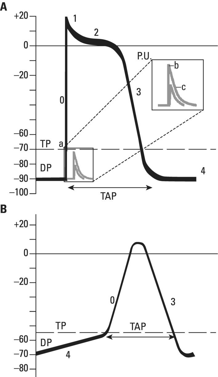
Depolarization (phase 0)


Repolarization (phases 1, 2, and 3)
In contractile cells
In slow response cells
Properties of cardiac cells
Automaticity
Excitability
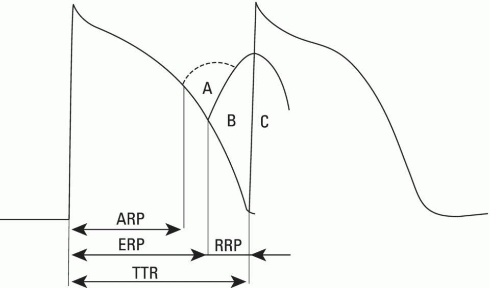
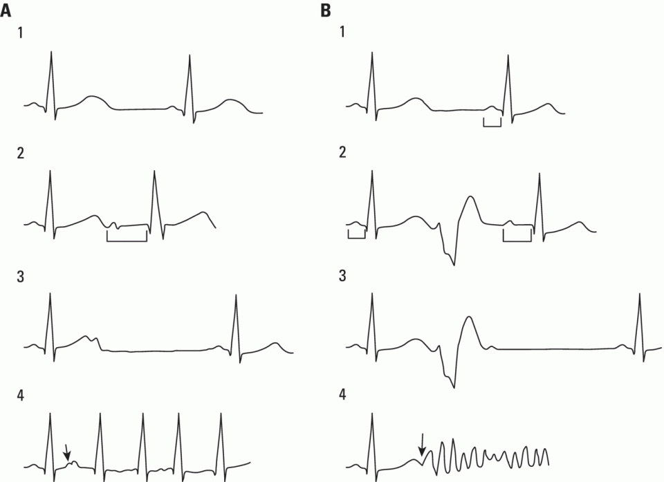
Refractory period
Rapid (fast) response cells
Slow response cells
Location
Mainly atrial and ventricular muscle and intraventricular conduction system
Sinus node, and to a lesser degree, AV node and mitral and tricuspid rings
Level of the DTP (diastolic transmembrane potential) and types of DTP (stable or unstable)
From −80 to −95 mV. The DTP is stable in contractile cells, but in the His–Purkinje cells there is a slight diastolic depolarization and the DTP is not completely stable
About −70 mV at onset. The DTP is unstable, presenting an ascendant curve which is characteristic of the automatic structures (e.g. sinus node)
Threshold level
About −70 mV
Less than −55 mV
Phase 0 upstroke
Rapid
Slow
Height of phase 0
High, reaches +20 to +40 mV
Low, reaches 0 to +15 mV
Conduction speed
Rapid (0.5–5 m/s)
Slow (0.01–0.1 m/s)
Fast sodium channels
Present
Absent
Slow channels, mainly for Ca2+ (and some Na+)
Present
Present
Inhibition of depolarization
By tetrodotoxin (puffer fish toxin), which inhibits fast Na channels
Manganese, cobalt, nickel, verapamil, etc., which inactivate slow Ca–Na channels
Duration of the effective refractory period (and consequently, recuperation of excitability) AB = Distance after depolarization, during which the cell is unexcitable
AB = Somewhat inferior to TAP duration (voltage‐dependent recuperation of excitability) (TAP = transmembrane action potential) 
AB = Superior to TAP duration (time‐dependent recuperation of excitability) 
Conductivity
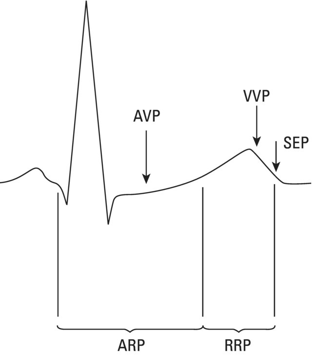
Vulnerability

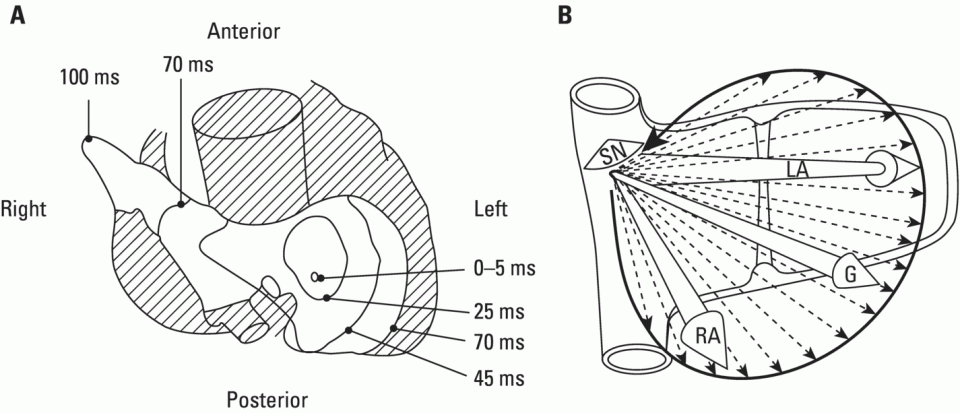
Cardiac activation
The normal origin of cardiac impulses: The sinus node
Atrial activation: The P loop
Atrial depolarization

 ) (see Figure 5.17).
Atrial repolarization
 ). The polarity of the atrial repolarization wave (ST–Ta) is therefore the opposite of that of the P wave. This wave is of very low voltage and longer duration than the P wave and is generally concealed by the superimposed QRS complex. Only in cases of AV block, atrial infarction, important right atrial enlargement, or sympathetic overdrive is it sometimes evident.
Transmission of the atrial impulse to the ventricle

Ventricular activation: QRS and T loops
Ventricular depolarization
Stay updated, free articles. Join our Telegram channel

Full access? Get Clinical Tree


