Segmented Poincaré Plot Analysis and Lagged Segmented Poincaré Plot Analysis

, Chandan Karmakar³, Michael Brennan³, Andreas Voss⁴ and Marimuthu Palaniswami³

(1)

Department of Biomedical Engineering, Khalifa University, Abu Dhabi, UAE

(2)

Department of Electrical and Electronic Engineering, The University of Melbourne, Melbourne, VIC, Australia

(3)

Electrical and Electronic Engineering, The University of Melbourne, Melbourne, VIC, Australia

(4)

Department of Medical Engineering and Biotechnology, University of Applied Sciences Jena, Jena, Germany

Abstract

Traditional Poincaré plot analysis (PPA) represents a two-dimensional graphical and quantitative representation of a time series dynamics. However, traditional PPA indices measure mainly linear aspects of the heart rate variability (HRV).

Therefore, we introduced a new method of PPA – the segmented Poincaré plot analysis (SPPA) that retains essential nonlinear characteristics of the HRV and other time series.

Additional insights into the underlying physiological mechanisms have been gained by extending the methodology of SPPA. Thus we developed the lagged SPPA (LSPPA) that investigates time correlations of the BBI.

For the first time we could demonstrate that an HRV index from SPPA was able to contribute to risk stratification in patients suffering from DCM. LSPPA provides a prognostic preview for DCM patients regarding several associated symptoms such as endothelial dysfunctions and increased risk stratification in DCM to 92% accuracy.

SPPA was also applied to BBI time series and blood pressure signals to investigate the coupling between those two time series.

In several studies we could demonstrate that the applications of SPPA and LSPPA lead to much more information about impaired autonomic regulation and have the potential to be applied in much more fields of medical diagnosis and risk stratification.

6.1 Introduction

Traditional Poincaré plot analysis (PPA) [59, 87, 89, 91] represents a two-dimensional graphical and quantitative representation of a time series dynamics. Babloyantz and Destexhe [170] were the first to introduce this nonlinear method for heart rate variability (HRV) analysis including both the pseudo-phase space and phase space quantification methods. Two-dimensional pseudo-phase space plots represent univariate system behaviour investigating signal values (N N _n + 1) as a function of their previous ones (N N _n), whereas phase space plots represent multivariate system behaviour investigating interactions of at least two different signals.

Typically the following indices from PPA are calculated: short-term (SD1) and long-term (SD2) fluctuations of the investigated system and the ratio SD1 ∕ SD2 [87, 89]. An ellipse can be drawn into the plot along the line of identity whereas the centre represents the mean value of the time series and the axes are SD1 and SD2. Even PPA is a nonlinear method where these indices appear insensitive to the nonlinear characteristics of the beat-to-beat intervals (BBI) [112].

Previous studies of patients suffering from dilated cardiomyopathy (DCM) have not evaluated the contribution of traditional PPA in risk stratification for sudden death [171, 172]. One reason for this is that these PPA indices measure mainly linear aspects of the BBI. Therefore, we recently introduced an enhanced method of PPA—the segmented Poincaré plot analysis (SPPA) [173] that retains essential nonlinear characteristics of the HRV time series. SPPA is characterized by a rotated and segmented Poincaré plot into a grid of 12 ×12 rectangles based on the centre of the cloud of points. Each rectangle is adapted to the SD1 (height) and SD2 (width).

In this chapter the ability of SPPA to differentiate between linear, nonlinear and Gaussian noise-caused dependencies is first tested by simulating and analysing such BBI time series. Then, surrogate analysis is performed to prove the ability of SPPA to obtain nonlinear behaviour in time series. Further, we represent a first study to investigate high- and low-risk patients suffering from DCM which subsequently use an extended SPPA method to investigate the Poincaré plot in a more detailed way by dividing the plot into 24 ×24 rectangles (adapted to SD1/2 and SD2/2) as well as into 48 ×48 rectangles (adapted to SD1/4 and SD2/4). Following this, SPPA will be performed to investigate age dependencies in healthy subjects.

The next step will be to apply SPPA to other cardiovascular signals such as systolic blood pressure (SBP) and diastolic blood pressure (DBP) in pregnant women suffering from hypertensive pregnancy disorders such as chronic or gestational hypertension and pre-eclampsia.

Even if the SPPA increases risk stratification [173], it still provides less information about the physiological background of the impaired autonomous regulation. Therefore, the objective was to investigate if time correlations will provide such information. As a consequence, the Lagged SPPA (LSPPA) method was developed to provide high-resolution analysis particularly in the very low (VLF = 0.0033–0.04 Hz) and low-frequency (LF = 0.04–0.15 Hz) bands [174]. In contrast to the traditional linear methods of HRV analysis [172, 175] and to PPA (related to BBIs) [172] which did not contribute to risk stratification, indices from LSPPA enhance risk stratification and provide some additional insights into the underlying physiological mechanism of heart rate regulation which will be later discussed.

Finally, we will discuss newer studies as well as first concepts to further improve these kinds of analysis methods to open up new fields of application. In this context, we will investigate other bio-signals such as respiratory signals and enhance the analysis method by introducing the interaction analysis using two-dimensional (2D SPPA) and three-dimensional (3D SPPA) approaches. This method improvement could lead to further enhanced information concerning alterations produced by coupled physiological systems.

6.2 Segmented Poincaré Plot Analysis

6.2.1 SPPA Method

The SPPA retains nonlinear features from a system based on PPA, representing an enhanced pseudo-phase space quantification method [173]. The Poincaré plots are two-dimensional graphical representations (as a cloud of points) of a time series plotted against its subsequent one. The calculation of PPA standard indices provides the basis for SPPA.

The SPPA method functions as follows:

The linear indices of SD1 and SD2 (Fig. 6.1a), representing short- and long-term fluctuations of the investigated system, are calculated according to traditional PPA (Eqs. 6.1–6.4), where Var is the variance, N N _nis a value of the time series with $n = 1,\ldots,N - 1$ (N is the length of time series) and N N _n + mis the shifted version of the same time series shifted by a lag of m = 1 [89, 112, 176]:

$\displaystyle\begin{array}{rcl} N_{n}& =& (NN_{1},NN_{2},\ldots,NN_{N-1}) {}\end{array}$

(6.1)

$\displaystyle\begin{array}{rcl} NN_{n+1}& =& (NN_{2},NN_{3},\ldots,NN_{N}) {}\end{array}$

(6.2)

$\displaystyle\begin{array}{rcl} \mathit{SD1}& =& \ \sqrt{\mathrm{VAR } \left (\frac{NN _{n } - NN _{n+1 } } {\sqrt{2}} \right )} {}\end{array}$

(6.3)

$\displaystyle\begin{array}{rcl} \mathit{SD2}& =& \ \sqrt{\mathrm{VAR } \left (\frac{NN _{n } + NN _{n+1 } } {\sqrt{2}} \right )}. {}\end{array}$

(6.4)

The cloud of points presented by PPA is then rotated α = 45^∘ around the main focus of the plot (Eq. 6.5), allowing for a simplified SD1 ∕ SD2 adapted probability-estimating procedure (Fig. 6.1b), whereby z is the axis of rotation and $\overline{NN_{n}}$ and $\overline{NN_{n+1}}$ are the mean values of the original (N N _n) and shifted versions (N N _n + 1) of a time series, respectively:

Fig. 6.1

The principle of SPPA; (a) traditional Poincaré plot, the calculation of SD1 and SD2; (b) rotated Poincaré plot (45^∘); (c) a segmented Poincaré plot including SPPA indices

$\displaystyle\begin{array}{rcl} \left [\begin{array}{c} NN_{n}^{\prime} \\ NN_{n+1}^{\prime} \\ {z}^{\prime}\end{array} \right ] = \left [\begin{array}{c} \overline{NN_{n}} \\ \overline{NN_{n+1}} \\ z\end{array} \right ] + \left (\left [\begin{array}{ccc} \cos \alpha &-\sin \alpha &0\\ \sin \alpha & \cos \alpha &0 \\ 0& 0 &1\\ \end{array} \right ] \times \left [\begin{array}{c} NN_{n} -\overline{NN_{n}} \\ NN_{n+1} -\overline{NN_{n+1}} \\ z\\ \end{array} \right ]\right ).& & {}\end{array}$

(6.5)

Starting from the centre of the cloud of points, a grid of 12 ×12 rectangles (Fig. 6.1c) is drawn into the plot. The size of each rectangle is adapted to SD1 (height) and SD2 (width).

The number of points within each rectangle (M _{i j}) related to the total number of points (N) was counted to obtain the single probabilities (p _{i j}). Based on these probabilities, all row (i) and column (j) probabilities were calculated by summation of the related single probabilities (Eqs. 6.6 and 6.7):

$\displaystyle\begin{array}{rcl} p_{ri}& =& \sum _{j=1}^{12}p_{ ij} {}\end{array}$

(6.6)

$\displaystyle\begin{array}{rcl} p_{cj}& =& \sum _{i=1}^{12}p_{ ij}. {}\end{array}$

(6.7)

6.2.2 Applying SPPA on Simulated BBI Time Series

The ability of SPPA to discriminate between different system states can be demonstrated with simulated time series. To compare SPPA to PPA, different BBI time series were simulated that are characterized by similar values of PPA indices SD1 and SD1. The four simulated time series were:

S1: Noise

Normal distributed white noise (Gaussian noise):

$\displaystyle{ h\left (x\right ) = \frac{1} {\sqrt{2\pi {\delta }^{2}}} {\ast}{\mathrm{e}}^{-\frac{{(x-\Delta x)}^{2}} {2{{\ast}\delta }^{2}} }. }$

(6.8)
S2: Nonlinear signal

Lorenz attractor:

$\displaystyle\begin{array}{rcl} \mathrm{d}x& =& (-\sigma x +\sigma y)\mathrm{d}t {}\end{array}$

(6.9)

$\displaystyle\begin{array}{rcl} \mathrm{d}y& =& (\rho x - y - xz) {}\end{array}$

(6.10)

$\displaystyle\begin{array}{rcl} \mathrm{d}z& =& (-\beta z + xy)\mathrm{d}t. {}\end{array}$

(6.11)
S3: Linear/nonlinear noisy signal

Three sinusoidal functions with Gaussian noise and Lorenz attractor:

$\displaystyle\begin{array}{rcl} x(t) = S1+S2+\mathrm{sin}(0.2 {\ast} 2 {\ast} pi {\ast} t)+\mathrm{sin}(0.15 {\ast} 2 {\ast} pi {\ast} t)+\mathrm{sin}(0.01 {\ast} 2 {\ast} pi {\ast} t).& & {}\end{array}$

(6.12)
S4: Linear surrogated noisy signal

Three sinusoidal functions with Gaussian noise and the surrogated Lorenz attractor:

$\displaystyle\begin{array}{rcl} x(t)& =& S1 + \mathrm{surrogate}(S2) + \mathrm{sin}(0.2 {\ast} 2 {\ast} pi {\ast} t) \\ & & +\,\,\mathrm{sin}(0.15 {\ast} 2 {\ast} pi {\ast} t) + \mathrm{sin}(0.01 {\ast} 2 {\ast} pi {\ast} t). {}\end{array}$

(6.13)

Applying the amplitude adjusted Fourier transform (AAFT) algorithm introduced by Theiler et al. [160], we generated surrogate time series which have the amplitude distribution and the power spectrum of the original BBI time series. The idea of the AAFT algorithm is to first rescale the values in the original time series to make them Gaussian. Then the Fourier transform (FT) algorithm is used to create surrogate time series including the same Fourier spectrum as the rescaled data. Finally, the Gaussian surrogate is rescaled back to have the same amplitude distribution as the original time series. A significant difference between the nonlinear values for the original and the surrogate time series shows that SPPA can reliably distinguish linear from nonlinear time series (see also Sect. 6.2.3). Therefore, we compare S3 (as the original signal including nonlinearities) with S4 (the surrogated signal) where S4 differs from S3 only in the surrogated part of the Lorenz signal part (S2).

The simulated BBI time series (S1–S4) were generated for t = 30 min each with a sampling frequency of 1,000 Hz (Fig. 6.2). Physiological properties somewhat representing human HRV were simulated by including sinusoidal signals of the most prominent frequency bands H F (0.2 Hz), L F (0.15 Hz) and V L F (0.01 Hz) with regard to the coupled signals S3 and S4. Additionally, the amplitudes of the signals have been adjusted without suppressing any dependencies within the coupled signals and ensuring similar linear indices calculated by traditional PPA as much as possible.

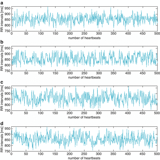
Fig. 6.2

Simulated BBI time series: (a) S1: Gaussian noise; (b) S2: Lorenz attractor; (c) S3: linear/ nonlinear noisy signal including three sinusoidal functions (0.2 Hz, 0.15 Hz and 0.01 Hz) with Gaussian noise and Lorenz attractor; (d) S4: linear surrogated noisy signal including three sinus functions (0.2 Hz, 0.15 Hz and 0.01 Hz) with Gaussian noise and the surrogated Lorenz attractor

In relation to the totalized value of amplitudes concerning all simulated BBI time series (S1–S4), we generated percentage amplitudes, respectively (Gaussian noise (S1, S3, S4): 4%; Lorenz attractor (S2–S4): 70%; sinusoidal functions (S3, S4): 14%).

Validating the defined dependencies within the simulated BBI time series, we applied the auto correlation function (ACF), which investigates linear dependencies, and the auto mutual information function (AMIF), which investigates linear and nonlinear dependencies in the simulated BBI time series (see Fig. 6.3). The concept of mutual information is based on an assessment of information flow I, defined by means of a probability distribution p [177–179] in the case of a discrete random number.

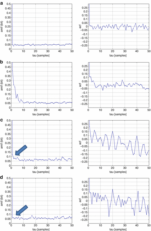
Fig. 6.3

Results of AMIF (left) and ACF (right) applying simulated BBI time series, respectively: (a) S1: Gaussian noise; (b) S2: Lorenz attractor; (c) S3: linear/ nonlinear noisy signal including three sinusoidal functions (0.2 Hz, 0.15 Hz and 0.01 Hz) with Gaussian noise and Lorenz attractor; (d) S4: linear surrogated noisy signal including three sinus functions (0.2 Hz, 0.15 Hz and 0.01 Hz) with Gaussian noise and the surrogated Lorenz attractor; the arrow highlights the different behaviour of the (surrogated) Lorenz attractor

In Gaussian noise, both functions are almost zero for each τ except for τ = 0 (S1—Fig. 6.3a). In case of pure nonlinearity (S2—Fig. 6.3b) and the nonlinear coupled time series (S3—Fig. 6.3c), significant nonlinear dependencies in the AMIF which are too wide peaks at τ = 0 can been shown. The arrows in Fig. 6.3c, d (S4) show the difference between the coupled time series. While the nonlinear part (Lorenz attractor) within S3 causes a wide peak, S4 does not exhibit this peak because of the destroyed nonlinear structures within the surrogated Lorenz attractor. In ACF a few linear dependencies can be shown in which S3 and S4 are coupled with three sinus functions.

The simulated BBI time series are presented in pseudo-phase space plots (Fig. 6.4), applying SPPA. This method provides a grid of 12 ×12 rectangles and a size adapted to SD1 and SD2 was applied (see also Sect. 6.2.1).

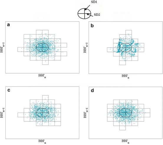
Fig. 6.4

SPPA plots applying simulated BBI time series: (a) S1: Gaussian noise; (b) S2: Lorenz attractor; (c) S3: linear/nonlinear noisy signal including three sinusoidal functions (0.2 Hz, 0.15 Hz and 0.01 Hz) with Gaussian noise and Lorenz attractor; (d) S4: linear surrogated noisy signal including three sinus functions (0.2 Hz, 0.15 Hz and 0.01 Hz) with Gaussian noise and the surrogated Lorenz attractor

The shape of the cloud of points concerning Gaussian noise (S1—Fig. 6.4a) and nonlinear Lorenz attractor (S2—Fig. 6.4b) is typical for these dependencies. The coupled signals are barely distinguishable (S3—Fig. 6.4c and S4—Fig. 6.4d).

Differences in SPPA are shown in spite of similar linear PPA indices. Mean deviations of 0.14% (mean value of BBI), 6.21% (SD1), 14.95% (SD2) and 12.81% (SD1 ∕ SD2) were reached when applying traditional PPA.

In addition, we calculated the row and column probabilities of the simulated BBI time series by applying SPPA. With regard to column 6 and rows 5–8, we calculated lower mean deviations (2.76–6.73%) by applying SPPA as compared to the traditional PPA. However, there are considerably higher mean deviations with regard to columns 3–5 (19.20–73.32%) and 7–10 (16.85–66.67%) as well as row 3 (67.41%), 4 (19.38%), 9 (24.04%) and 10 (66.67%).

To summarize, we could achieve considerably higher mean deviations by applying SPPA (2.76–73.32%) as compared to PPA (0.14–14.95%), confirming the assumption of SPPA to increase the differentiation between various dependencies such as Gaussian noise, nonlinearity and several coupled signals.

6.2.3 The Ability of SPPA to Obtain Nonlinear Behaviour in Time Series When Applying Surrogate Data Analysis

As previously mentioned in Sect. 6.2.2, surrogate data analysis techniques are applied, testing nonlinearity in time series by constructing surrogate data sets. Therefore, the AAFT algorithm described by Theiler et al. [160] is used to destroy nonlinear structures within time series while linear structures are maintained.

The aim of the following surrogate analysis is to test the ability of SPPA to obtain nonlinear structures represented in nonlinear BBI time series. In this study, 20 surrogate time series were generated by shuffling an original BBI time series.

The surrogate data analysis technique is applied for simulated nonlinear BBI time series (S2: Lorenz attractor—Sect. 6.2.2) consisting of three nonlinear parts (Eqs. 6.9–6.11). To illustrate the dependencies within the investigated BBI time series, the behaviour of two linear PPA indices (SD1 and SD2—see Fig. 6.5) and one nonlinear SPPA index (fourth column—Fig. 6.6) are shown as an example. Thus, the figures represent the value of the original BBI time series compared to the values of the surrogated BBI time series, respectively.

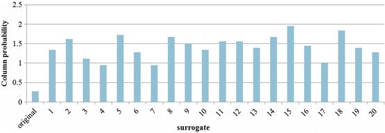
Fig. 6.5

Traditional linear PPA indices (SD1 and SD2) applying the original nonlinear BBI time series (Lorenz attractor) and its 20 surrogated BBI time series each

Fig. 6.6

Typical SPPA indices (column 4) applying the original nonlinear BBI time series (Lorenz attractor) and its 20 surrogated BBI time series

It could be shown that linear indices (SD1 and SD2) exhibit small deviations especially in relation to the value of the original BBI time series as compared to the nonlinear index (column 4), which presents significantly higher deviations.

Table 6.1 represents SPPA and traditional PPA indices by applying the original nonlinear BBI time series as well as the averaged one applying 20 surrogate BBI time series, whereas the most important indices are marked which significantly discriminate high- and low-risk DCM patients in a subsequent study applying the lagged segmented Poincaré plot analysis (LSPPA—see also Sect. 6.4.2).

Table 6.1

Column and row occurrences applying the most important SPPA and PPA indices investigating the original simulated BBI time series (Lorenz attractor) and the averaged mean value of BBI and its standard deviation (SD), calculating 20 surrogated BBI time series; the difference in % specifies the deviation between the original index and its averaged surrogated BBI time series; significant LSPPA indices are marked

			Surrogate
Method	Indices	Original	Mean BBI	SD	Difference in %
SPPA	Column 3	0.0000	0.0000	0.0000	0.00
	Column 4	0.2781	1.3745	0.3421	79.77
	Column 5	19.4105	15.4535	0.5934	20.39
	Column 6	33.9822	34.1208	0.9934	0.41
	Column 7	25.5840	32.2259	1.2327	20.61
	Column 8	19.5217	14.0623	0.8743	27.97
	Column 9	1.2236	2.7462	0.4657	55.44
	Column 10	0.0000	0.0167	0.0408	100.00
	Row 3	0.1112	0.0083	0.0204	92.50
	Row 4	1.3904	2.1536	0.2075	35.44
	Row 5	14.9055	14.4713	0.6289	2.91
	Row 6	34.3715	33.3695	0.4916	2.92
	Row 7	32.9255	33.3528	0.4625	1.28
	Row 8	14.5718	14.4741	0.6482	0.67
	Row 9	1.6129	2.1619	0.2271	25.40
	Row 10	0.1112	0.0083	0.0204	92.50
PPA	Mean	857.7575	857.7144	0.0211	0.01
	SD1	35.0760	36.2740	1.1795	3.30
	SD2	39.3134	38.0830	1.0708	3.13
	SD1 ∕ SD2	0.8922	0.9540	0.0569	6.48

Calculating the deviations of surrogate BBI time series (SD1 = 35. 08 ± 0. 024; SD2 = 39. 31 ± 0. 021) and the original BBI time series (SD1 = 35. 07; SD2 = 39. 31), we obtained small ones when applying PPA (difference: 0.001–0.009%). In comparison, there are higher deviations (difference: 1.47–100%) when applying SPPA as seen by the representative example found in column 4 (original: 0.28; surrogate = 1. 43 ± 0. 28; difference: 80.53%). In conclusion, we could confirm that indices from PPA represent linear dependencies, whereas SPPA indices obtain nonlinear dependencies representing considerable differences, as seen by the selected nonlinear structures.

6.2.4 Application of SPPA for Risk Stratification in Dilated Cardiomyopathy Patients

DCM is a chronic disease of the heart muscle characterized initially by a dilated left ventricle or dilation of both ventricles. This is attached to normal or reduced wall thickness and an impaired systolic function [180]. In the industrialized countries with aging populations, DCM is one of the most common public health problems (mortality of 5% per year) and occurs much more frequently (1,856,000 patients in the USA [181]) than other major forms of cardiomyopathy [182].

Various studies were performed to indicate risk stratification in patients with DCM. In former studies it was demonstrated that linear and nonlinear methods of HRV and baroreflex sensitivity (BRS) analysis could not considerably contribute to risk stratification in those patients [175, 183]. Therefore, the aim of this study is to analyse the suitability of SPPA to improve the risk stratification in DCM patients.

We enrolled 91 DCM patients (70 male and 21 female) and 21 references (healthy subjects; REF). The diagnosis of all DCM patients was confirmed by experienced cardiologists using coronary angiography and echocardiography (Table 6.2). From every patient a thirty-minute high-resolution ECG (orthogonal corrected Frank lead ECG, 22-bit resolution, 1,600 Hz sampling frequency) was recorded.

Table 6.2

Classification of healthy subjects (REF) and DCM patients

	REF	DCM group	DCM_HR	DCM_LR
Number of subjects (male/female)	21 (12/9)	91 (70/21)	14 (11/3)	77 (59/18)
Age (year)	35 ± 13	55 ± 10	54 ± 11	56 ± 10
EF (%)	–	36 ± 12	31 ± 6	37 ± 12
NYHA (I-IV)	–	2. 2 ± 0. 8	2. 6 ± 0. 9	2. 1 ± 0. 8
LVEDD (mm)	–	63. 5 ± 8	68. 8 ± 10	62. 5 ± 7

After a two-year follow-up, the DCM patients were divided into two groups: DCM without progression of the disease (low-risk, DCM_LR) and patients who died due to a cardiac event or were reanimated because of a life-threatening arrhythmic event (high-risk, DCM_HR). BBI were extracted using self-developed wavelet-based pattern recognition software [172]. The ECGs and the patients’ data were stored in a database. A heart rate time series (tachogram) consisting of successive BBI were extracted from the ECG data. Applying an adaptive variance estimation algorithm, ectopic beats and artefacts were rejected and interpolated. These disturbances could considerably influence the PPA and, in particular, the SPPA [173, 183].

The nonparametric Mann-Whitney U-test was performed to determine the highly significant indices (p < 0. 01) and the significant indices (0. 01 ≤ p < 0. 05), differentiating between DCM patients and healthy subjects as well as between high-risk and low-risk DCM patients. The receiver operating characteristic (ROC) was computed univariate as well as multivariate, estimating the sensitivity for each value vs. the specificity. To validate a specific method, the performance of each index was assessed by estimating the area under the ROC curve (AUC).

Former studies of ECG could not improve risk stratification in patients suffering from DCM [171, 172]. The aim of this method is to prove the ability for both discrimination between DCM_HR and DCM_LR and between DCM and REF, as well as to perform basic testing for LSPPA. The results of the group tests applying SPPA are demonstrated in Table 6.3.

Table 6.3

Most significant SPPA indices discriminating DCM_HR vs. DCM_LR and DCM vs. REF including mean values and their SD in normalized row and column probabilities of occurrences; sensitivity (SENS), specificity (SPEC) and AUC (N.S. not significant; *p < 0. 05; **p < 0. 01)

	p (DCM_LR vs. DCM_HR)	p (DCM vs. REF)	Mean ± SD in % (DCM_HR)	Mean ± SD in % (DCM_LR)	Mean ± SD in % (REF)	SENS in %	SPEC in %	AUC in %
Column 4	N.S.	0.0014**	2. 41 ± 1. 10	2. 12 ± 1. 03	1. 68 ± 0. 63
Column 5	0.0241*	N.S.	12. 01 ± 2. 81	14. 16 ± 2. 93	13. 12 ± 2. 45	67.5	64.3	69.0
Column 8	0.0005**	N.S.	12. 63 ± 2. 10	14. 42 ± 1. 20	13. 59 ± 2. 42	75.3	71.4	80.0
Row 9	N.S.	0.0002**	1. 76 ± 0. 63	1. 55 ± 0. 71	1. 14 ± 0. 64	71.4	68.1	76.6
Row 10	N.S.	0.0007**	0. 26 ± 0. 18	0. 23 ± 0. 19	0. 11 ± 0. 14	76.2	67.0	73.9
Row 11	N.S.	0.0052**	0. 06 ± 0. 05	0. 04 ± 0. 06	0. 01 ± 0. 03	81.0	49.5	67.8

SPPA partly discriminates between the investigated groups. Highly significant indices of the group test between DCM patients and REF could be calculated as seen in columns 4 (p = 0. 0014), 9 (p = 0. 0002) and 10 (p = 0. 0007) and in row 11 (p = 0. 0052). One significant index (column 5: p = 0. 0241) and one highly significant index (column 8: p = 0. 0005) could be determined as risk predictors in DCM patients differentiating between DCM_HR and DCM_LR. Therefore, column 8 represents the highest AUC value of 80.0% with a sensitivity of 75.3% and a specificity of 71.4%.

The highest significant columns (columns 5 and 8) for risk stratification in DCM patients are shown in Fig. 6.7 and are exemplary for DCM_HR and DCM_LR patients, respectively.

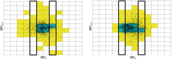
Fig. 6.7

Examples of SPPA plots applying DCM_HR (left) and DCM_LR (right) patients, respectively; yellow marked rectangles generally include measuring points and the blue ones exhibit a single probability of more than 5%; the most significant columns 5 and 8 are framed

The percentage of measuring points within the highly significant columns is higher in DCM_HR patients (column 5: mean = 1. 223 ± 0. 124; column 8: mean = 1. 249 ± 0. 106) than in DCM_LR patients (column 5: mean = 0. 990 ± 0. 214; column 8: mean = 1. 021 ± 0. 167). This means a higher dispersion of measuring points in patients with DCM_HR when compared to DCM_LR patients of DCM.

The highly significant columns (5 and 8) are located at a distance of SD2 apart, the mean of both BBI_n(mean_BBI_n). In general, the borders of the highly significant columns can be described as follows:

Column 5: from mean_BBI_n − 2 * SD2 to mean_BBI_n − SD2
Column 8: from mean_BBI_n + 2 * SD2 to mean_BBI_n + SD2

The distance between the centre of the cloud of points and the significant columns of SPPA (columns 5 and 8) is equal in both directions (SD2). The significant columns are ranged very symmetrically around the centre of the cloud of points. Przibille et al. [184] were the first to study the influence of the standard deviation of all BBI (SDNN) within the Poincaré plots. Therefore, it could be shown that patients with an SDNN < 50 ms died due to a cardiac event. They identified HRV analysis as being highly significant for DCM patients [184]. In our study, we found no significant differences in SDNN investigating high- and low-risk DCM patients, but highly differences discriminating between DCM patients and healthy subjects. These differences are caused probably due to the considerable limitations and the low number of enrolled patients in the compared study.

In conclusion, for the first time HRV indices from PPA were able to contribute to risk stratification (AUC value of 80.0%) in patients suffering from DCM. Further on, the SPPA retains nonlinear features, and therefore, overcomes limitations of traditional PPA.

6.2.5 Investigating the Influence of Rectangle Size

The standard SPPA method (see Sect. 6.2.1) fits a grid of 12 ×12 rectangles into the cloud of points where the size of the rectangles is adapted to the standard deviations SD1 and SD2. Investigating the influence of the rectangles’ size, we decreased the size of the rectangles by a half (SD1/2, SD2/2) or quarter (SD1/4, SD2/4), leading to an increased number of rectangles within the Poincaré plot.

In order to demonstrate SPPA’s performance related to the varying rectangle sizes, we investigated DCM patients (idiopathic DCM) as introduced in Sect. 6.2.4.

Test Method I

The size of the rectangles is adapted to SD1 ∕ 2 and SD2 ∕ 2, increasing the number of rectangles to 24 ×24 rectangles (Fig. 6.8a).

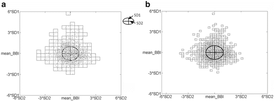
Fig. 6.8

Additional SPPA plots with different rectangle sizes; (a) test method I: SD1 ∕ 2, SD2 ∕ 2 and 24 ×24 rectangles; (b) test method II: SD1 ∕ 4, SD2 ∕ 4 and 48 ×48 rectangles

Table 6.4 presents significant columns of the BBI time series applying test method I. The coloured columns are located within the highly significant columns of standard SPPA. Therefore, column 10 (test method I: p = 0. 0441) is located within column 5 (blue-coloured) and column 16 (test method I: p = 0. 0008) in column 8 (red-coloured) of standard SPPA, as pictured in Fig. 6.9.

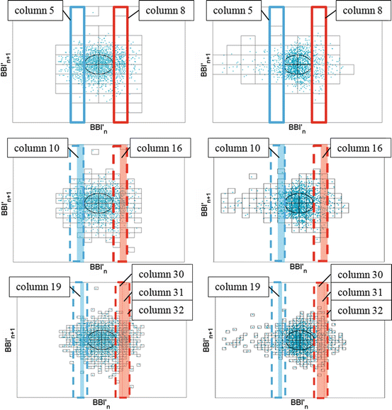
Table 6.4

Significant indices applying test method I including the mean value and SD for the group test DCM_HR vs. DCM_LR (N.S. not significant; *p < 0. 05; **p < 0. 01)

Fig. 6.9

Illustration of significant columns regarding standard SPPA (top), test method I (middle) and test method II (bottom) investigating DCM HR (left) and DCM LR (right)

Additionally, columns 4 (p = 0. 0336) and 5 (p = 0. 0071) could discriminate between the investigated groups of patients when applying test method I.

Test Method II

Test method II quadruples the number of rectangles in comparison to the standard SPPA. Therefore, the size of the rectangles is adapted to SD1 ∕ 4, SD2 ∕ 4, thus dividing the Poincaré plot into 48 ×48 rectangles (Fig. 6.8b).

Table 6.5 represents significant columns as a result of test method II and discriminating between DCM_HR and DCM_LR patients. Therefore, the coloured columns are part of highly significant columns of standard SPPA. To this end, test method II was assigned four different columns: column 19 (p = 0. 004) located within column 5 (blue-coloured) and columns 30 (p = 0. 004), 31 (p = 0. 001) and 32 (p = 0. 024) assigned within column 8 (red-coloured) of standard SPPA, also pictured in Fig. 6.9.

Table 6.5

Significant indices as a result of test method II for the group test DCM_HR vs. DCM_LR (N.S. not significant; *p < 0. 05; **p < 0. 01)

Furthermore, we calculated three significant columns (column 9: p = 0. 014, column 10: p = 0. 018 and column 11: p = 0. 024) located within column 3 of standard SPPA.

Therefore, it could be concluded that the results of test method I and test method II are rather similar to the results of standard SPPA.

6.2.6 Investigating Age Dependencies in Healthy Subjects

Even HRV analysis is an established method for characterizing autonomic regulation [114, 185–187] and has various applications [158, 188–197]. The demands for short-term HRV analysis are continually increasing, especially in the ambulatory sector, to monitor temporary examinations and to obtain an almost immediate test result. There is a great demand for short-term HRV analysis methods determining reference values of linear and nonlinear short-term HRV indices from a healthy population when considering age and sex dependencies.

The objectives of this study are to generally investigate age dependencies of short-term HRV indices and to investigate this age dependency over the course of several decades in healthy subjects [198].

The present study includes 12-lead ECG signals (based on KORA S4 study [199]) recorded under resting conditions over a period of 5 min (sample frequency 500 Hz). The investigated subjects were informed about their participation. Furthermore, the study conforms to the recommendations of the Declaration of Helsinki and has been approved by the appropriate medical ethics committee. A total of 1,906 ECG recordings from healthy subjects were selected consisting of 782 women and 1,124 men between the ages of 25 and 74 years (see Table 6.6).

Table 6.6

Classification of healthy subjects within each age class (2 and 5 age classes)