Fig. 1.1
Pulse-echo principle. A pulse of sound of known frequency is generated and emitted in a known direction. The echoes returning from an object can be used to derive information regarding the object, including distance, size, etc.
The following sections discuss the physical process in which ultrasound, specifically through the use of the pulse-echo principle, is utilized to obtain detailed information for medical diagnostic imaging—particularly in regard to noninvasive cardiac evaluation by echocardiography, including TEE.
Physics of Sound and Ultrasound
Sound: Definition and Properties
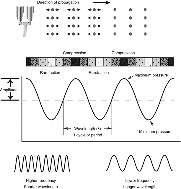
Sound is a form of mechanical energy that requires a physical medium for transmission; this medium must contain molecules (such as air, water, etc.) that are used to propagate the sound. Unlike electromagnetic waves, which do not require a medium for propagation, sound cannot be transmitted in a vacuum. A sound wave is created when a discrete source—a vibrating or oscillating object—pushes and pulls adjacent molecules, causing them in turn to vibrate; this vibration spreads to adjacent molecules, and thus a disturbance is propagated away from the source in the form of a longitudinal wave characterized by a series of back and forth vibrations of molecules (Fig. 1.2). The direction of this back and forth vibration is parallel to the direction of wave propagation. The wave that is created represents a series of compressions, when the molecules are pushed together, and rarefactions, when the molecules are pulled apart (Fig. 1.2). If one could measure the instantaneous pressure at different points, the regions of compression, in which there is a greater density of molecules, would have a higher pressure than normal, and the regions of rarefaction (with a lesser density) would have a lower pressure than normal. Plotting a graph of pressure vs. distance from the source (along the line of propagation) would produce a curve in the shape of a sine wave (Fig. 1.2). The importance of this sine wave is that, like any wave, it has certain properties that can be used to describe it. The peak of one wave to the next peak (or valley to valley) represents one full wave or one complete cycle or period; the number of times per second that the cycle is repeated is termed the frequency, and the unit to measure this is cycles per second, or Hertz (Hz). This frequency is determined by the number of oscillations per second made by the sound source. The physical distance between two peaks (or valleys) is termed the wavelength and often designated by the symbol λ. This is the distance the sound wave travels in one complete cycle. The importance here is that frequency and wavelength are inversely related, and their magnitude depends upon the speed of sound in the medium (Table 1.1A). The equation relating these three variables is given as follows:

(1.1)
λ = wavelength
c = speed of sound in the medium
f = frequency in cycles/second
Fig. 1.2
Generation of a sound wave. A vibrating source (in this case, a tuning fork) causes adjacent air molecules to vibrate in a back-and-forth direction. This oscillating motion propagates away from the source in a series of compressions and rarefactions; when the air pressure at any one point is plotted as a function of time, a sine wave is obtained with a wavelength (λ) and pressure amplitude (P). Shorter wavelengths are associated with higher wave frequencies; longer wavelengths with lower frequencies. This example shows sound propagation in air, but the same principles apply in water or in the soft tissue of the human body
Fig. 1.3
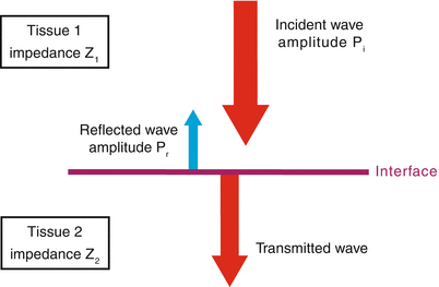
Specular reflection. When an incident sound wave of amplitude Pi encounters a smooth interface perpendicular to the direction of propagation, some is reflected (amplitude Pr) and the remainder transmitted. The degree of transmission vs. reflection depends upon the relative differences in acoustic impedance between the two tissues (Z1 and Z2)—the greater the impedance mismatch, the greater the amount of sound reflected
Table 1.1
Physical properties of sound for various tissues in the human body
A. Speed of sound | |
Material | Speed of sound (m/s) |
Lung | 600 |
Fat | 1,460 |
Liver | 1,555 |
Blood | 1,560 |
Kidney | 1,565 |
Muscle | 1,600 |
Lens of eye | 1,620 |
Skull bone | 4,080 |
B. Acoustic impedance | |
Tissue | Acoustic impedance (Rayls × 10−4) |
Air | 0.0004 |
Lung | 0.18 |
Water | 1.5 |
Brain | 1.55 |
Blood | 1.61 |
Liver | 1.65 |
Kidney | 1.62 |
Human soft tissue, mean | 1.63 |
Muscle | 1.71 |
Skull bone | 7.8 |
C. Attenuation coefficient | |
Tissue | Attenuation coefficient (dB/cm) |
Water | 0.0022 |
Blood | 0.18 |
Brain | 0.85 |
Liver | 0.9 |
Fat | 0.6 |
Kidney | 1.0 |
Muscle | 1.2 |
Skull bone | 20 |
Lung | 40 |
The speed of sound varies depending upon the medium: the denser the medium, the faster the speed of propagation. In biological systems, the speed of sound exhibits wide variation: it is lowest in the lungs, which are air-filled structures (about 600 m/s), and highest in bone (about 4,080 m/s) (Table 1.1A). In the soft tissues, the average speed of sound is about 1,540 m/s, and this is the number generally used when calibrating the range-measuring circuits of most diagnostic ultrasound instrumentation [1]. As will be shown throughout this chapter, the speed of sound in the human body plays an important role in a number of considerations related to echocardiography.
The importance of Eq. 1.1 is that, by knowing the speed of sound in the medium, the wavelength can be calculated for a given sound frequency, and vice-versa. The range of sound frequencies audible by the human ear is between 20 and 20,000 Hz. However, if sound waves of these frequencies were transmitted in the body, the corresponding wavelengths would be far too large for use in the medical field. For diagnostic medical imaging, adequate resolution is possible only when the wavelength of the sound wave is comparable to the size of the smallest objects being imaged [6, 7]. For echocardiography, this translates to millimeters or less, which means that sound frequencies in the millions of Hertz (megahertz, or MHz) must be used. Note that these frequencies are extremely high, several orders of magnitude beyond the range of human hearing—hence the term ultrasound. Echocardiography generally utilizes frequencies between 1 and 15 MHz, which by Eq. 1.1 yields a wavelength between 0.1 mm (15 MHz) and 1.54 mm (1 MHz). The higher the frequency, the smaller the wavelength, and the better the spatial resolution.
The other important property of a sound wave is its amplitude, which describes the strength of the wave, or maximum pressure elevation from baseline (Fig. 1.2). This corresponds to the “loudness” of the sound. This property, also known as acoustic pressure, is measured in Pascals (P). The amplitude of the sound represents the energy associated with the sound wave: the more the energy, the “louder” the sound and the greater the amplitude. Another parameter used to express the “loudness” of the sound is known as intensity. This term is used to describe the energy flowing a cross-sectional area per second and is proportional to the square of acoustic pressure, as noted by the equation:

(1.2)
I = intensity
P = acoustic pressure in Pascals
ρ = density of the medium
c = speed of sound in the medium
Intensity is the parameter used to characterize the spatial distribution of ultrasound energy. As noted, it describes the amount of ultrasonic power per unit area (given in watts/square meter, or more commonly milliwatts per square centimeter), and can vary depending upon location. The difference between acoustical power and intensity can be illustrated in the following example: two beams (one focused, one unfocused) are emitted with the same acoustic power. While the unfocused beam has a more uniform distribution of energy; the focused beam will produce more concentrated energy in the area focused. Hence, the intensity is greater in that area. Intensity is also one of the parameters used to evaluate the biological effects of ultrasound. At sufficiently high intensities and long enough exposure times, ultrasound can produce a measurable effect on tissues, notably in the form of heating and cavitation (tiny bubbles from dissolved gases in the medium) [1]. The subject of the biological effects of ultrasound on human tissue is beyond the scope of this chapter. Suffice it to say that while no known ill effects have been noted from the intensity levels and scan times commonly used in diagnostic medical ultrasound, it is still important to be mindful of the remote possibility—particularly if equipment manufacturers were to increase output intensities to improve imaging [3, 8].
For medical imaging, a standard method for quantifying intensities or power levels is to use the decibel (dB) system. Instead of providing an absolute number, this method produces a value that represents a relative change (or ratio) between two amplitudes or two intensities. Using two echo signal intensities I 1 and I 2 or two echo signal amplitudes A 1 and A 2 (I 1 and A 1 representing the reference signal), the signal level in dB is calculated as follows:
(1.3)
It is meaningless to use a dB level as an absolute value. Rather, the dB notation provides a value obtained when comparing a particular intensity or amplitude to a reference value. In diagnostic medical ultrasound, the transmitted signal generally serves as the reference value. Note that the dB represents a logarithmic scale, therefore an intensity change of +3 dB represents a doubling of intensity, and −3 dB a halving of intensity. The dB system is used to express output power, dynamic range, or ultrasonic attenuation in tissue (see below). It represents a simpler, more compact method to express large differences in power levels or intensity, and will be used throughout the remainder of this chapter.
Reflection: The Key to Ultrasonic Imaging
As an ultrasound wave propagates through the body, several different interactions are possible as it encounters the various tissues interfaces. These interactions, analogous to those occurring with light waves, include: (a) continued transmission, (b) reflection, (c) refraction, (d) absorption. Of these, reflection is the key interaction that makes possible the generation of ultrasonographic/echocardiographic information. As mentioned above, diagnostic medical ultrasound consists of emitting sound pulses in a known direction, and then collecting and processing the returning echo signals—that is, the signals that have been reflected from the various internal structures in the body (in the case of echocardiography, the heart, blood, and vascular structures). The differences in the strength of the returning signals enable the ultrasound machine to build an image of the various tissues, as well as the tissue-tissue and tissue-blood interfaces, and this forms the basis of echocardiographic imaging. What determines how echo signals are reflected, and the strength of these signals? A fundamental factor is acoustic impedance, an intrinsic property of tissue that characterizes its capacity for sound transmission. The acoustic impedance of a tissue is directly proportional to its underlying density—the denser the tissue, the higher the acoustic impedance. Each type of tissue has a different acoustic impedance: air has an extremely low impedance, bone has a very high impedance, and the various soft tissues have impedances that differ from each other but vary within a much narrower range (Table 1.1B). At a tissue interface, the degree of reflection vs. transmission of an incident sound wave depends upon the relative difference in acoustic impedance between the two tissues—that is, the degree of impedance matching. When there is a small impedance mismatch, most of the sound energy is transmitted, and only a small amount is reflected and returns to the source (transducer) to be used as imaging information (Fig. 1.3). As the transmitted energy continues further, some is reflected in a similar manner at more distant interfaces, yielding imaging information from deeper structures. This process continues along the length of the ultrasound beam. In this manner, ultrasonic information is progressively obtained, and imaging is possible to significant depths because the acoustic impedance differences are small for most soft tissue-soft tissue interfaces. However, if a significant impedance mismatch exists between two tissues, then virtually all sound is reflected, and very little transmitted. Almost no usable information is available beyond the interface (a phenomenon known as “acoustic shadowing”). This is the reason that lung interferes with ultrasonic imaging: it is not that ultrasound cannot propagate through lung, it is that the impedance mismatch is so great between lung and soft tissue that virtually all ultrasound energy is reflected. It is also the reason that ultrasonic gel is used with transthoracic imaging: to improve the acoustic coupling (impedance matching) between the transducer and the chest wall.
Acoustic impedance matching is important whenever a sound wave encounters an interface between two tissues, and it is particularly important for those interfaces that are much larger than the size of the ultrasound wavelength. When such interfaces are large and smooth, they are termed specular reflectors and they behave like a large acoustic mirror (speculum = mirror in Latin). If there is a sizable impedance mismatch, incident ultrasound beams will undergo a great deal of reflection. If the incident beam is directed perpendicular to the surface, the reflected sound waves return to the transducer as a well-defined, redirected beam (echo), leading to a very bright appearance on the display screen (Fig. 1.4). If the incident ultrasound beam strikes the specular reflector at an angle, the reflected portion will be directed at an angle θ r which is equal to the incident angle θ i but in the opposite direction. The remainder of the incident beam that is transmitted can be “bent” or refracted, with the amount of refraction depending upon the difference between the speed of sound between the two tissues, as given by Snell’s Law (Fig. 1.5). The greater the difference in the speed of sound between the two tissues, the greater the degree of refraction. Again, this is analogous to the behavior of light waves. In general, refraction is not a major problem with diagnostic ultrasound because there is little variation in the speed of sound among the soft tissues in the human body. However in certain situations, refraction can lead to image errors; this can be seen in the setting of interfaces between fat and soft tissue.
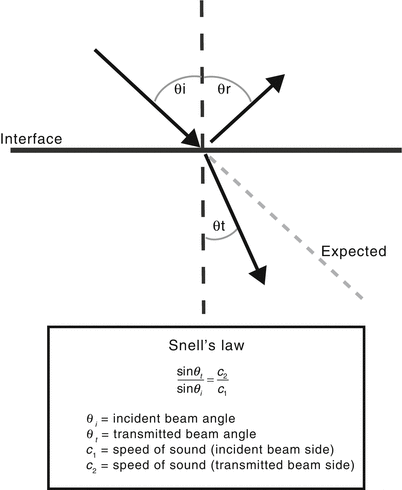
Fig. 1.4
Example of a large specular reflector (diaphragm) and acoustic scattering produced by imaging of the liver (a) and myocardium (b). Note that the echoes from the specular reflector have the largest amplitude (brightness) when the surface is perpendicular to the angle of insonation. In (b), the myocardium has the characteristic heterogeneous 2D appearance produced by natural acoustic reflections and interference patterns (scattering) from its various components, also known as “speckle”
Fig. 1.5
Refraction and Snell’s law. When the incident sound wave encounters a large specular reflector at a nonperpendicular angle θ i (θ i refers to the angle as measured from the perpendicular axis), the reflected beam travels off at an equivalent angle θ r. The transmitted wave undergoes refraction or “bending”. The amount of refraction can be predicted by Snell’s law, which is itself based upon the difference in the speed of sound between the two tissues. The greater the difference, the greater the degree of refraction
What if the large surface is not smooth, but rough? In this case the uneven surface causes incident energy to be reflected in a number of different directions. This is called diffuse reflection (Fig. 1.6). Such reflections can cause a loss of beam coherence and a weaker echo returning to the transducer. Some organ boundaries, as well as the walls of the heart chambers (irregular endocardial surfaces), fall within this category. At first glance, it would appear that that these signals, along with the nonperpendicular signals to a specular reflector (whether reflected at an angle or refracted) would not be as useful for imaging because they are not directed back to the transducer. However in practice, even these off-angle specular and diffuse reflectors are useful for ultrasonic imaging due to the range to different transducer positions that can be utilized. In addition, divergences of the ultrasound beam can result in sound waves that will be reflected back to the transducer [9]. In fact, echoes from diffuse reflectors, while weaker, can be useful because of the fact that they are not as sensitive to the orientation of the transducer.
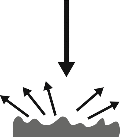
Fig. 1.6
Diffuse reflector. An incident beam striking a rough, uneven surface results in lower amplitude reflected waves that travel away from the reflector in multiple directions. This type of echo is not as dependent upon interface orientation as a specular reflector
The information from diffuse and specular reflectors is most useful at the boundaries of objects and organs, for example along the diaphragm or pericardium. However an even more important type of reflection accounts for much of the useful diagnostic information in ultrasonic imaging, including echocardiography. This type of reflection is called acoustic scattering, also known as nonspecular reflection. It refers to reflections from objects the size of the ultrasound wavelength or smaller. The parenchyma of most organs, including the heart, contains a number of objects (reflectors) of this size. The signals from these reflectors return to the transducer through multiple pathways. The sound from such reflectors is no longer a coherent beam; it is instead the sum of a number of component waves that produces a complex pattern of constructive and destructive interference. This interference pattern is known as “speckle” and provides the characteristic ultrasonic appearance of complex tissue such as myocardium (Fig. 1.4a) [7]. These signals tend to be weaker, and echo signal strength varies depending upon the degree of scattering. The degree of scattering is primarily based upon: (a) number of scatterers per unit volume; (b) acoustic impedance changes at the scatterer interfaces; (c) size of the scatterer—increased size produces increased scattering; (d) ultrasonic frequency—scattering increases with increasing frequency/decreasing wavelength [1]. The last point is important, because it contrasts to specular reflection, which is frequency independent. Therefore it is possible to enhance scattering selectively over specular reflection by using higher ultrasound frequencies. Also, because of the fact that scattering occurs in multiple directions, the incident beam angle/direction is not as important as with specular reflectors. This is why organ parenchyma (such as liver) can be readily viewed from a number of different transducer positions (Fig. 1.4b). Changes in scattering amplitude will result in brightness changes on the ultrasound image on the display, giving rise to the terms hyperechoic (increased scattering, brighter) and hypoechoic (decreased scattering, darker), and anechoic (no scattering, black appearance).
At the opposite extreme from the large specular reflectors are the very small reflectors whose dimensions are much less than the ultrasonic wavelength. Such reflectors also produce scattering, and are termed Rayleigh scatterers. This category most notably includes red blood cells, and the scattering that results from these gives rise to the echo signals from blood for Doppler and color flow imaging. Scattering from Rayleigh scatterers increases exponentially (to the fourth power) as frequency is increased.
Attenuation and Ultrasonic Imaging
As ultrasound travels through tissue, the amplitude and intensity of the signal decreases as a function of distance. This is known as attenuation, and is due to several mechanisms. The first mechanism is one in which acoustic energy is converted into another form of energy, principally heat; this is known as absorption. The second mechanism involves redirection of beam energy, by a number of different processes including scattering, reflection, refraction, diffraction, and divergence (the latter two processes result in a spreading of the sound beam). Scattering and reflection (and also refraction) were discussed above; while both play an essential role in diagnostic medical imaging, each process also reduces the intensity of ultrasound energy transmitted distally, thereby attenuating the transmitted signal. The third mechanism involves interaction between sound waves, known as interference. Wave interference occurs when two waves meet. It can be constructive or destructive, depending upon whether the two waves are in phase or out of phase. When in phase (constructive), an additive effect is produced, increasing amplitude; when out of phase (destructive), the waves can effectively cancel each other out. The degree of attenuation can be given as an attenuation coefficient (α) in decibels per centimeter (dB/cm), representing the reduction in signal amplitude or intensity as a function of distance. The amount of attenuation, as measured in decibels, can be calculated by the equation: Attenuation (dB) = α × distance (cm). The attenuation coefficient varies with the type of medium through which the ultrasound is transmitted (Table 1.1C). As can be seen, there is little attenuation in blood, but significant attenuation in bone. Attenuation in muscle is twice that of other tissues such as liver. Another important determinant of attenuation is the frequency of the ultrasound beam. In most cases, attenuation increases approximately linearly with frequency: the higher the frequency, the greater the attenuation (Fig. 1.7).
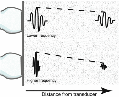
Fig. 1.7
Attenuation of ultrasound in parenchyma. As an ultrasound pulse travels through tissue, its amplitude and intensity decrease as a function of distance from the transducer. This is known as attenuation. Higher frequency sound waves are attenuated much more rapidly than lower frequencies
However, as will be seen with much of ultrasound, there are tradeoffs. In this particular case, the tradeoff is depth. While higher frequencies provide enhanced spatial resolution, in soft tissue they are attenuated much more rapidly than lower frequencies, hence the depth of penetration is much less, and so the higher frequencies are not as useful for visualizing deeper structures. This is why higher frequency, higher resolution transthoracic imaging is much more feasible in pediatric compared to adult patients. It is also one of the reasons that TEE provides superior imaging compared to transthoracic imaging in larger patients: the proximity of the esophagus to the heart significantly reduces attenuation and enables the use of higher frequency ultrasonic imaging.
Important Principles of Echocardiographic Image Formation
At first glance, the basic premise behind 2D imaging in echocardiography seems relatively straightforward. Using the pulse-echo principle discussed above, an ultrasound pulse is emitted as a well-directed beam, and reflected echo signals are collected from the beam line. If this is continued while the ultrasound beam is swept in an arc (sector), a 2D image can be constructed, using echo arrival times and beam axis location to determine the precise location of reflectors within the sector (Fig. 1.8).
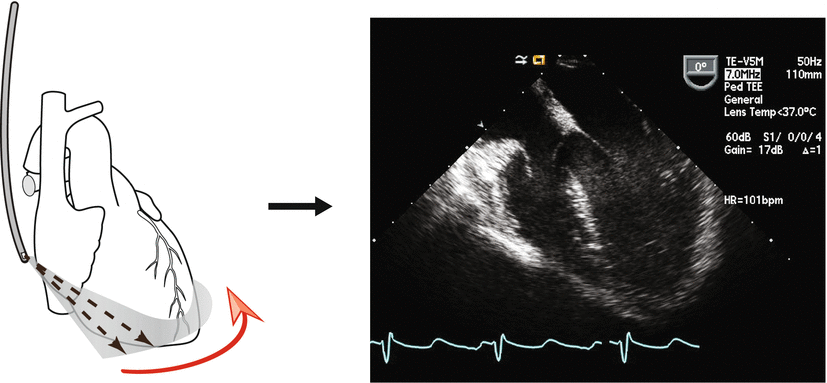
Fig. 1.8
Production of an ultrasound (echocardiographic) image. A pulse of ultrasound is transmitted in a well defined beam, and the transducer “listens” while echoes are received from the same beam path. These echoes appear as dots (brightness) corresponding to signal amplitude. During 2D imaging, the beam is swept across a sector (red arrow), and displaying all the beams along this sector results in a two-dimensional (B-mode) image. In this example, a transesophageal transducer is shown, but the same process occurs with transthoracic echocardiography
However, the actual process by which reflected ultrasound signals are converted into real-time, 2D echocardiographic images is deceptively complex, requiring sophisticated and technologically intricate hardware, along with highly advanced and powerful computing and digital signal processing capabilities. A number of different steps are involved: generation of high quality and well-directed ultrasound pulses, reception and digitization of the returning signals, multilayered digital signal processing, and conversion of these signals to a real-time 2D image of sufficient medical diagnostic quality (while at the same allowing operator manipulation and pre/post processing of the images). Moreover, for echocardiography and TEE the same process must be repeated rapidly and continuously in order to display the real time motion of the heart.
The sections that follow discuss the process by which ultrasound pulse generation leads to image formation, specifically as pertains to echocardiography. For simplicity’s sake, the discussion will first cover basic ultrasound beam forming principles utilizing single element transducers. These principles will then be applied to array transducers, which form the basis for modern day echocardiography, including TEE.
Transducers
The first step in ultrasound imaging requires the creation and transmission of an appropriate sound wave; this is accomplished by the use of a transducer. Technically, the term transducer refers to any device that is used to convert one form of energy into another. The ultrasonic transducer converts electrical energy to mechanical (acoustic) energy in the form of sound waves that are then transmitted into the medium. When reflected sound waves return, the reverse process occurs: the transducer receives the acoustic energy and converts it into electrical signals for processing. Transducers in medical ultrasound achieve this conversion by the piezoelectric (PZE) effect. The PZE effect is a special property seen with certain types of crystals (quartz, ceramics, etc.). When an electrical signal is applied to such a crystal, it vibrates at a natural resonant frequency, sending a sound wave into the medium. Conversely, acoustic energy received by the crystal produces mechanical pressure or stress, which then causes the crystal to generate an electrical charge that can be amplified, yielding a useful electrical signal. Thus PZE transducers can serve as both detectors and transmitters of ultrasound. As noted previously, the signals must be appropriate for imaging of tissues in the human body—wavelengths must be no more than 1–2 mm, which means sound frequencies must be in the millions of Hertz. While several PZE crystals found in nature (e.g. quartz) have been used for ultrasonography, most present day ultrasound transducers utilize man-made PZE ceramic (such as lead zirconate titanate, also known as PZT) and composite ceramic elements. When excited, these PZE elements can produce the very high frequencies required for diagnostic medical imaging. A PZE transducer operates best at its natural resonance frequency, which corresponds to the crystal (element) thickness; however newer composite elements have wide frequency bandwidths and can operate at different frequencies, enabling generation of multiple frequencies from one transducer. In these instances, the native frequency, which usually represents the midpoint of the frequency distribution, is termed the “center” or “central carrier” frequency.
However, a transducer is not simply a housing surrounding a PZE element or collection of elements (see arrays below). While the PZE element serves as the most important component of an ultrasound transducer, a number of other essential components also reside in the transducer. These include backing (damping) material, electrodes, an insulating cover, housing, matching layer, and acoustic lens (in some transducers) (Fig. 1.9). The matching layer, which covers and attaches to the PZE element, is very important because of the significant impedance mismatch that exists between the PZE element and surface (skin or esophagus). The matching layer contains an acoustic impedance intermediate between the two surfaces; this helps to match impedances from one surface to the other, allowing for efficient sound transmission between transducer element and soft tissue. In some transducers, multiple matching layers are used to facilitate transmission of a range of ultrasound frequencies. Also, newer composite PZE elements have acoustic impedances much closer to that of soft tissue.
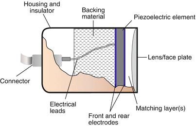
Fig. 1.9
Diagram of a single element transducer. The various components of the transducer are seen. In this example, there is a large, single piezoelectric crystal. For an array transducer, instead of a large single element, multiple elements would be laid in a single row, each with its own electrical connector. However the other parts of the transducer would be analogous to the single element transducer
The backing (damping) material also serves an important role. Pulse-echo ultrasound involves the transmission of a short pulse of sound, followed by a period in which the transducer “listens” for the returning echoes. As it turns out, for ultrasound imaging the transducer spends only a tiny fraction of time actually transmitting sound—this is known as the duty factor, and typically comprises less than 1 % of the total time. The rest of the time is spent listening for returning echoes. For this to occur, the transducer can emit only a very short pulse of acoustic energy, usually a small number of cycles in length. To produce these, short bursts of electrical energy cause the PZE element to vibrate or “ring”, which generates the acoustic pulse. The length of the pulse train, also known as pulse duration or spatial pulse length, is truncated by damping the duration of the vibration as quickly as possible, and the backing material plays an important role here. An important point regarding pulse duration is that short pulses are desirable to optimize axial resolution, as will be discussed below. The typical pulse length is 1–3 cycles in length. Of note, a shorter pulse is a less “pure” tone, and contains a wider range of frequencies, also known as having a broader bandwidth (Fig. 1.10). This range of frequencies encompasses the labeled operating (center) frequency, which represents the midpoint of the frequency distribution. Wide bandwidth associated with short pulse duration is more desirable for imaging applications; narrower frequency bandwidth associated with longer pulse duration is more useful for pulsed Doppler applications.
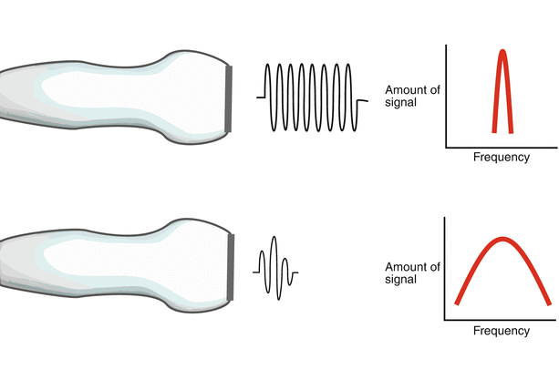
Fig. 1.10
Spatial pulse length. The top pulse has undergone less damping; therefore it has a longer duration, or spatial pulse length, and a purer “tone” with most of the sound at or near a certain frequency. Contrast this with the bottom pulse, which has undergone excellent damping that reduces the spatial pulse length. This type of pulse is characterized by a large frequency bandwidth
Transducer Beam Formation and Geometry
When sound waves originate from a single, small point source whose size is similar to the wavelengths it produces (such as a bell), the waves radiate outward in all directions (Fig. 1.11a). However this results in an unfocused signal, unsuitable for medical imaging in which a directed, focused ultrasound beam becomes considerably more important. Diagnostic medical ultrasound transducers are designed to direct ultrasound pulses in a specific direction. A single element ultrasound source of large dimension (for example, a transducer face much larger than the wavelength of sound emanating from it) can produce equally spaced, linear wavefronts (Fig. 1.11b) also known as planar wavefronts [10]. Conceptually, these planar wavefronts can be described as a collection of multiple individual point sources, also known as Huygen sources, and the wavelets arising from these sources are known as Huygen wavelets [1]. Interference among wavelets results in the large planar waveform (Fig. 1.11c).
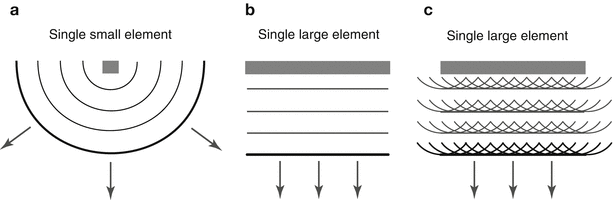
Fig. 1.11
Sound wave geometry. (a) A single small element has a size similar to the wavelength it produces. Sound from this element radiates in all directions. (b) The single element is much larger than the sound wavelengths it produces, resulting in equally spaced, planar wavefronts. These planar wavefronts can be thought of as a collection of individual point sources, each with its own wavelet. These are known as Huygen wavelets (c)
One of the important aspects of ultrasound beam formation concerns the geometry of the beam and its impact upon imaging. With a single element, unfocused ultrasound transducer, the individual wavelets from a transducer form a near parallel beam wave front, as noted in Fig. 1.11c. Two important zones develop in this beam. The first distance is the near field, or Fresnel zone. This area is characterized by many regions of constructive and destructive interference, leading to fluctuations in intensity. In this zone, the beam remains well collimated for a certain distance, and even narrows slightly (Fig. 1.12). Beyond the near field, the beam diverges, and some energy escapes along the periphery of the beam; this is known as the far field or Fraunhofer zone (Fig. 1.12). Fresnel (near-field) length is directly proportional to aperture of the transducer element and inversely proportional to transducer frequency, as given by the equation:
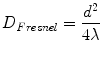
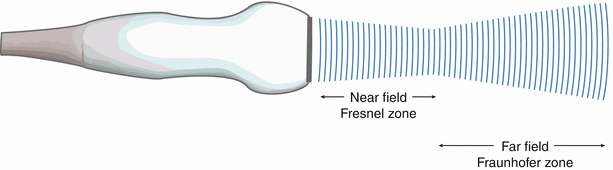

(1.4)
D Fresnel = Fresnel (near field) length
d = diameter, or aperture, of the transducer
λ = ultrasound wavelength
Fig. 1.12
Sound beam pattern from a single element, unfocused transducer. The near field is known as the Fresnel zone, the far field is known as the Fraunhofer zone. Note that the sound beam is well collimated in the near field and diverges in the far field
The importance of these two zones lies in the fact that lateral resolution is best before divergence of the beam, hence the best imaging and spatial detail are obtained within the Fresnel zone, or near-field. From Eq. 1.4, it becomes apparent that a larger transducer diameter as well as higher frequencies (leading to shorter wavelengths) will increase the near field length and maximize image quality (Fig. 1.13). These have an immediate impact on lateral resolution.
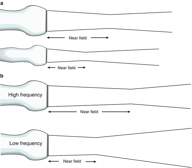
Fig. 1.13
Effect of transducer frequency and diameter on near field length. (a) Both transducers have the same frequency but the larger diameter transducer has a longer near field length, and less beam divergence. (b) Both transducers have the same diameter, but the transducer with the higher frequency has the longer near field length and less beam divergence
The above considerations of frequency and transducer diameter were discussed in the context of a single element, unfocused transducer. It is clear that—even without beam focusing—it is desirable to perform imaging in the near field. However there is another very important aspect of beam geometry: that of focusing the beam, which has the effect of narrowing the beam profile. The narrowest portion of this beam is the focal distance, and the focal zone corresponds to the region over which the width of the beam is less than two times the beam width at the focal distance (Fig. 1.14). This is the area in which ultrasound intensity is highest, and also where the lateral resolution is best; whenever possible, imaging of key structures should be performed within this zone. As will be discussed below, a focused, narrow beam is desirable for 2D imaging. With single element transducers, this is performed by utilizing a curved PZE element or acoustic lens to focus and narrow the beam width; however in such cases the focal distance is generally fixed. Nonetheless in the past these focused, single element transducers formed the basis of the early mechanical sector echocardiography platforms. Obviously the ability to change a transmit focus dynamically would enhance the imaging capabilities of an ultrasound platform. The advent of array technology marked a significant advance in the field of echocardiography: variable beam focusing and beam shaping became a reality, adding a great deal of flexibility and versatility to echocardiographic imaging. Array technology is discussed in the next section.
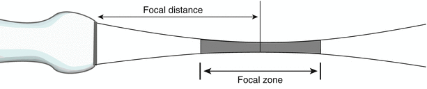
Fig. 1.14
Beam pattern for a focused transducer. The beam is narrowest at the focal distance, hence the best lateral resolution is within the focal zone. Focusing can either be done externally (e.g. acoustic lens) for a single element transducer or, in the case of an array transducer, focusing can be performed electronically and dynamically
Arrays
The foundation of current ultrasound transducer technology, particularly that used in echocardiography, is built upon the concept of transducer arrays. Rather than a single element, an array consists of a group of closely spaced PZE elements, each with its own electrical connection to the ultrasound machine. This enables the array elements to be excited individually or in groups. The resultant sound beam emitted by the transducer results from a summation of the sound beams produced by the individual elements. The wave from an individual element (which is quite small, often less than half a wavelength) is by itself broad and unfocused. However when a group of elements transmits simultaneously, there is reinforcement (constructive interference) of the waves along the beam direction, and cancellation (destructive interference) of the waves in other directions, yielding a more well-defined, planar ultrasound beam (Fig. 1.15a). The whole concept of arrays is based upon Huygens’ principle, in which a large ultrasound beam wavefront can be divided into a large number of point sources (Huygen sources) from which small diverging waves (Huygen wavelets) merge to form a planar wavefront [1]. The resultant beam can also be focused electronically by introducing time delays to the separate elements, in a manner essentially the same as using a focusing lens or curved PZE element (Fig. 1.15b). Electronic beam steering can occur, in which beams can be swept across an imaged field without any mechanical motion in the transducer (unlike the older mechanical sector transducers). Moreover the focal distance is not fixed but dynamic, and can be adjusted by the operator. Furthermore, multiple transmit focal zones can be utilized to increase the focal zone of an instrument, thereby improving image quality throughout the sector (however this requires extra “pulses” and can result in a lower image frame rate). Thus the array transducer provides a tremendous amount of flexibility for imaging.
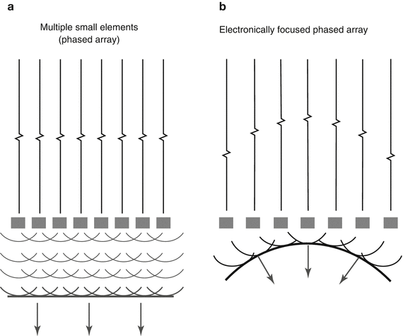
Fig. 1.15
Phased array transducer. When all elements are stimulated simultaneously, the waves from the individual elements act as Huygen point sources, merging to produce a large planar wavefront (a). With an array transducer, the beam can be focused by introducing time delays to the separate elements (b), producing beam geometry analogous to that obtained by an acoustic lens
There are a number of different types of arrays available for ultrasonic imaging (linear, curvilinear, annular), but the phased array transducer is generally the one used for 2D transthoracic and transesophageal echocardiography. This type of array is smaller than linear and curvilinear arrays, thereby providing a transducer “footprint” that allows the transducers to be used with the smaller windows available for transthoracic (particularly pediatric) and transesophageal imaging. The number of PZE elements in a transthoracic phased array probe generally ranges between 64 and 256 (or more) elements. One of the important distinguishing characteristics of phased array transducers is that—unlike linear and curvilinear arrays—all elements of the phased array are excited during the production of one transmitted beam line (Fig. 1.16). The direction of the beam is steered electronically by varying the timing sequence of excitation pulses; the term phasing describes the control of the timing of PZE element excitation in order to steer and focus the ultrasound beam. In this manner, timing sequence alterations allow successive beam lines to be generated (Fig. 1.16). Therefore in phased array transducers, the beam can be electronically swept in an arc, providing a wide field of view despite the relatively small footprint. In addition, the direction of echo reception (“listening”) can be varied electronically. Returning echo signals from reflectors along each scan line are received by all the elements in the phased array; because of slightly different distances from a reflector to the individual elements, the returning signals will not be in phase and therefore electronic receive focusing must be performed to bring them back into phase to prevent destructive interference of returning signals. This is done by applying time delays to the individual element returning signals, analogous to the time delays used for transmission. In this way, the signals from the individual elements will be in phase when summed together to produce a single signal for each reflector. Receive focusing is adjusted dynamically and automatically by the ultrasound machine in order to compensate for different reflector depths.
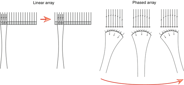
Fig. 1.16
Linear vs. phased array transducer. In the linear array, small groups of elements are stimulated to produce one beam line. Once the returning signals are received, a second adjacent group of elements is stimulated to produce the second beam line. This process continues sequentially down the length of the transducer. Not all elements are stimulated at one time. In contrast, the phased array transducer has a smaller footprint, and all elements are utilized to produce and steer every beam electronically. By varying the timing of pulses to the elements, sequential beam lines are generated and swept in an arc (red arrow under the right diagram)
An essential component of modern ultrasound systems that use array transducers is the beam former. This component of the system provides pulse-delay sequences to individual elements to achieve transmit focusing. In addition, it controls beam direction and dynamic focusing of received echoes, as well as other signal processing. It is located on the ultrasound system and electronically connected to the individual transducer PZE elements. Traditionally, beam formers have been analog, but most ultrasound manufacturers now utilize digital beam formers.
A newer type of array, the matrix array, has been developed for real-time three-dimensional (3D) transthoracic and transesophageal echocardiography. This consists of more than 2,500–3,000 elements laid out in a two-dimensional square array slightly larger than 50 × 50 elements [11] (Fig. 1.17). Analogous to 2D phased array, all elements in the matrix array are active during beam forming. Because of the large number of elements the process of beam forming is divided into two areas: (1) pre-beam forming by custom made integrated circuits within the transducer handle, and (2) traditional digital beam forming within the ultrasound system [12, 13]. The most important aspect of 3D beam forming is the ability to steer in both lateral and elevational directions, thereby providing a pyramidal 3D dataset. Three-dimensional technology and imaging (specifically in the context of 3D TEE) is discussed in Chap. 2 as well as Chaps. 19 and 20.
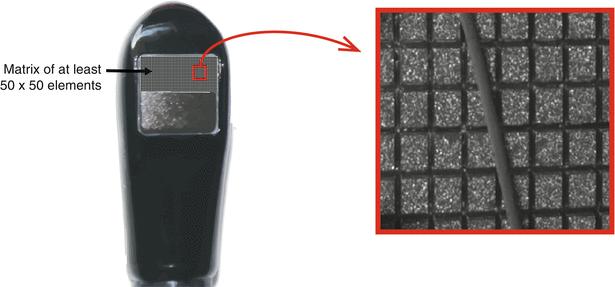
Fig. 1.17
Matrix array three-dimensional transesophageal echocardiography probe. The transducer is a square matrix of at least 50 × 50 elements (2,500–3,000 total elements). A pyramidal three dimensional dataset is produced from this. Each individual element is just larger than the diameter of a human hair (Photograph on the right, courtesy of Philips Medical Systems, Andover, MA)
Transesophageal Echocardiographic Transducers
All current 2D TEE probes utilize phased array technology, usually in a row of 64 elements for current adult multiplane TEE probes (some pediatric probes have fewer elements—see Chap. 2). TEE probes are constructed similar to standard transthoracic transducers: they have a collection of piezoelectric elements, backing material, electrical connector, housing, and matching layer. In addition an acoustic lens is added below the matching layer to improve focusing. The important difference is that all the components, as well as the housing, are much smaller, and special cabling is required for anterior/posterior flexion (anteflexion/retroflexion) and (in some probes) right/left rotation (Fig. 1.18). In addition, with multiplane TEE probes the piezoelectric elements can be electronically or mechanically rotated by cables (Fig. 1.18), a rotor, or even a small motor housed in the probe tip, and attached to the elements, allowing the tomographic plane to be varied between 0° and 180°. More detailed discussion of TEE technology is given in Chap. 2.
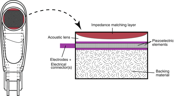
Fig. 1.18
Internal layout of model of a multiplane transesophageal echocardiographic (TEE) probe. The probe utilizes phased array technology; the transducer containing the array of elements is located at the probe tip and can be rotated between 0° and 180° by either an electronic or mechanical control in the probe handle. The principal transducer components (right diagram) are similar to those found in a transthoracic probe. Rotation of the transducer can be achieved using cables (as shown on left), a central rotor, or a small motor housed in the probe tip. The TEE probe itself is similar to a gastroscope, with controls in the probe handle (not shown, see Chap. 2) for tip movement anteriorly/posteriorly and right/left (Note: in some pediatric probes, the right/left control has been omitted)
Pulse Repetition Frequency
Ultimately, one of the major factors determining the quality of information obtained by ultrasonic imaging, particularly that of echocardiography, is the speed of sound in tissue. This generally fixed value imposes certain restrictions on pulse-echo imaging as well as pulsed wave and color flow Doppler evaluation—specifically, it places limits on the at maximum rate at which ultrasound pulses can be emitted. A transducer cannot send and receive ultrasound pulses at the same time; once a pulse has been sent, the transducer must wait a certain period of time for returning echoes, with the round-trip time depending upon the depth of the reflector. The equation relating distance to time is:

(1.5)
T = Time it takes a pulse of sound to travel to a reflector, and for an echo to return to the transducer (round-trip time)
D = Distance from the transducer
c = Speed of sound in the medium
Given a speed of sound in tissue of 1,540 m/s, the round-trip time is equivalent to 13 μs/cm of depth, hence the time needed to collect all returning echoes from a scan line of depth D is equal to 13 μs × D. This time is also known as the pulse repetition period, and the reciprocal of this is known as the pulse repetition frequency, or PRF. This is a very important concept in echocardiography, because the maximum PRF represents the maximum number of times a pulse can be emitted per second. PRF will vary with the speed of sound in different media. However, assuming a constant speed of sound (as is seen with soft tissues in the human body), PRF is totally dependent upon depth: the greater the depth, the less the maximum PRF. In the soft tissues of the human body, maximum PRF calculates to 77,000/s/cm of depth (roughly equivalent to 1 divided by 13 μs). Typically, PRF is expressed in units of Hz or kiloHz (kHz). For example, for a depth of 10 cm, the maximum PRF for one scan line will be 77,000 ÷ 10 cm, or 7,700/s (also given as 7,700 Hz or 7.7 kHz). In other words, for this particular depth, the maximum number of times a sound pulse can be transmitted and received is 7,700 times/s. As will be seen, the PRF plays an important role in determining the limits of temporal resolution for both 2D imaging as well as the maximum velocities measurable by pulsed wave and color flow Doppler.
Generation of an Echocardiographic Image
The pulse-echo principle serves as the fundamental concept underlying ultrasonic and echocardiographic imaging. This principle is based upon a predictable and reliable constant: the speed of sound in the soft tissues of the human body, which, as noted above, is 1,540 m/s. When an acoustic pulse is emitted by a transducer, the time delay between transmission and signal detection can be used to calculate distance from the transducer, by rearranging Eq. 1.5 above:

(1.6)
Thus for ultrasonography and echocardiography, it is axiomatic that time equals distance: the transmit/receive time (divided by 2) serves as the measurement for distance. Returning echoes along a scan line will have their various depths registered as a function of their time of return, as calculated by Eq. 1.6. In addition, these returning echoes will have different amplitudes that correspond to the different reflectors encountered. In the past, the amplitude of returning signals was displayed directly by an oscilloscope (known as “A–mode”). However, all modern-day echocardiography platforms convert the amplitude of returning echoes to a corresponding gray scale value for display on a computer monitor—this is known as brightness mode, or “B–mode”. By plotting these varying brightness points as a function of distance from the transducer, one scan line can be displayed. If successive scan lines are rapidly swept across the object of interest, a 2D image can then be assembled, with echo signal location on the display corresponding to the reflector positions in relation to the transducer (Fig. 1.19). As discussed previously, this scan line sweep is performed electronically with a phased array transducer, using time delay sequences to vary the activation of the individual elements and sequentially “steer” the scan lines. Typically, 100–200 separate scan lines are used for a single 2D image [3]. For echocardiography, this process must be repeated rapidly in order to depict accurate, real-time cardiac motion.
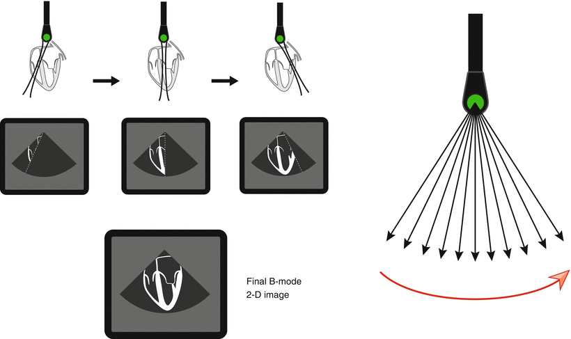
Fig. 1.19
Generation of a two dimensional (2D) echocardiographic image. The returning echo amplitudes from one scan line are converted to pixel gray scale brightness on a computer monitor. This is also known as “B-mode” (for brightness mode). If successive scan lines are obtained and rapidly swept across the sector, a 2D image can be generated (red arrow indicates the direction of the scan line sweep). This process must be repeated rapidly in order to depict accurate real-time cardiac motion
The process whereby the reflected echoes are converted to real-time, 2D echocardiographic images requires highly specialized and advanced technology, as well as sophisticated digital signal processing capabilities. Returning echo signals from reflectors along each scan line are received by all the phased array elements in the transducer; as noted previously, electronic receive focusing is performed to bring returning signals into phase. Analog to digital conversion also occurs during this process. To compensate for different reflector depths, this receive focusing is adjusted dynamically and automatically by the digital beam former. These digital signals are then sent to a receiver in the ultrasound machine, where they undergo a number of preprocessing steps to “condition” the signal; these include signal preamplification and demodulation, as well as operator-adjustable time gain compensation (TGC), noise reduction (known as reject), and dynamic range/compression (that varies contrast). The TGC is a selective form of amplification used to compensate for the weaker, attenuated signals from increased depths. Some of this can be performed by the operator, but modern echocardiography machines now incorporate an adaptive TGC that automatically adjusts the TGC in real-time [3]. The operator-adjusted TGC controls will be discussed in a separate section below.
Once the signals have been amplified and processed, they are sent to a scan converter, which is a digital imaging matrix used to store and buffer returning signal information. In the process, the returning echo signal locations are converted from polar to Cartesian coordinates—in other words, angle and depth information are converted to a matrix format for display on a computer monitor. A common setup is a matrix of 512 × 512 pixels, with each pixel having 8 bits of storage allowing 256 levels of gray scale (though other types of setup are possible) (Fig. 1.20). Location information is obtained from: (a) angle of the scan line in relation to a reference axis, which is parallel to the surface of the array elements; (b) distance from the scan line to the reflector, as calculated from Eq. 1.6 above. These two coordinates are then converted into Cartesian x and y coordinates, which can then be placed into a large rectangular matrix suitable for pixel mapping on a 2D computer display. What becomes apparent during this conversion process is that, when the scan lines are superimposed upon the matrix, adjacent scan lines will not sample all of the pixels in the matrix. To fill in these areas, a process of interpolation is performed in which an averaged signal from nearby pixels is used to fill in the value of the blank (unsampled) pixel (Fig. 1.20).
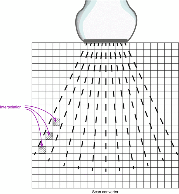
Fig. 1.20
Scan converter. The scan lines are converted from polar to Cartesian coordinates, and the information placed in a scan converter matrix, and used to construct a two dimensional image that can be visualized on a computer monitor. A common setup is a 525 × 525 pixel matrix, with each pixel having 8 bits of storage allowing 256 levels of gray scale. However, other matrix sizes and bits/pixels are possible. Interpolation is performed for those pixels in which no scan line information is available
In the scan converter, image data can be held in memory and continuously updated with new echo data. At the same time, information is continuously read out to a video buffer to provide real-time visualization of the scanned images on a video monitor. Most echocardiography systems now use a large digital computer monitor, generally one based upon liquid crystal display (LCD) technology. Various postprocessing techniques can also be performed on the digital image data stored in the computer memory; these techniques include contrast and edge enhancement, as well as smoothing and B-mode color. For echocardiography, image acquisition, updating, and display must occur in a rapid fashion to portray real-time cardiac motion. Almost all ultrasound systems also have a freeze option that stops image acquisition (still frame) and allows visualization of a single image (for measurements or text labeling), and also a review of short cine loops. This feature is very useful for echocardiography, because it provides the ability to slow down and review rapidly moving images associated with cardiac motion. It also facilitates visualization of the acquired data relative to the phases of the cardiac cycle as displayed by concurrent electrocardiographic monitoring.
Stay updated, free articles. Join our Telegram channel

Full access? Get Clinical Tree


