A multivariable logistic regression model conforms to the following formula:
![$$ Ln\;\left[p/\left(1-p\right)\right] = {A}_0+{A}_1\ast {X}_1+{A}_2\ast {X}_2+{A}_3\ast {X}_3\dots {A}_n\ast {X}_n $$](/wp-content/uploads/2017/02/A305677_1_En_15_Chapter_Equb.gif)
![$$ Ln\;\left[p/\left(1-p\right)\right] = {A}_0+{A}_1\ast {X}_1+{A}_2\ast {X}_2+{A}_3\ast {X}_3\dots {A}_n\ast {X}_n $$](/wp-content/uploads/2017/02/A305677_1_En_15_Chapter_Equb.gif)
In which A 0 is a constant, n is the number of explanatory variables, A n are the coefficients of determination, and X n are the explanatory variables in the model. X n can be a categorical (entry values: 0 or 1) or a continuous variable (entry value: absolute value of the variable or any specific variable transformation).
The odds ratio (OR) for a specific variable after adjusting for every other variable in the model, i.e., the increased mortality risk for each unit increase of the explanatory variable X n , is defined as
![$$ OR\left[ CI,p- value\right]={e}^{A_n} $$](/wp-content/uploads/2017/02/A305677_1_En_15_Chapter_Equc.gif)
![$$ OR\left[ CI,p- value\right]={e}^{A_n} $$](/wp-content/uploads/2017/02/A305677_1_En_15_Chapter_Equc.gif)
The CI (confidence interval) and the p-value determine the significance of the OR, namely, if the p-value shows statistical significance, a variation in the explanatory variable will have an effect in the response variable, provided the remaining variables remain constant.
15.2.3 Variable Selection
The variables entered in a risk model are commonly selected according to clinical principles; however, the number of variables selected has to be balanced to maximize the predictive power of the model. Too few variables can limit the predictive power by ignoring the effect of relevant unmeasured variables. Likewise, an excessive number of variables can create random error or noise, also called over-fitting, which prevents a model from being reproducible. The rule of ten in logistic regression suggests that the absolute number of the outcome event variable should be at least ten times the number of variables initially considered in a model, i.e., with 100 mortality events in a study sample, the model should not consider more than ten explanatory variables to avoid over-fitting (Peduzzi et al. 1996). Thus, although many institutional studies present risk-adjusted results, the majority lacks the necessary power to meet this requirement, and registry data is often necessary to obtain accurate ORs; this is particularly true in low-frequency outcome variables, such as operative mortality in cardiac surgery.
15.2.4 Risk Model Assessment
There are generally three steps in the assessment of the accuracy of a risk model. First, the model is tested for its performance across the spectrum of predicted probability of the outcome variable, also called calibration or goodness of fit. Furthermore, the sensitivity of the model to discriminate between positive or negative outcome events is measured, also called discrimination. Finally, the model undergoes “validation” by testing the goodness of fit and discrimination in a dataset comparable to the one used to create the model.
15.2.4.1 Goodness of Fit
The calibration or goodness of fit of a model is most commonly measured by the Hosmer–Lemeshow test, by which the study population is divided into ten equal-sized groups arranged from the lowest to the highest predicted probability of the outcome event. The observed and expected values for each of the two outcomes (e.g., death or survival) are entered in a contingency table, and the test statistic is used to determine whether there is a significant difference between the observed and expected values within each decile (Table 15.1). A p-value of >0.05 is generally accepted to indicate that the observed frequencies are similar to those predicted by the model, thus reflecting an adequate goodness of fit (Hosmer and Lemeshow 2000).
Table 15.1
Hosmer–Lemeshow contingency table
Decile group | Total events | Outcome event = 0 | Outcome event = 1 | ||
|---|---|---|---|---|---|
Observed events | Expected events | Observed events | Expected events | ||
1 | 100 | 95 | 92.1 | 5 | 7.9 |
2 | 100 | 93 | 90.3 | 7 | 9.7 |
3 | 100 | 93 | 93.1 | 7 | 6.9 |
4 | 100 | 91 | 92.5 | 9 | 7.5 |
5 | 100 | 90 | 88.3 | 10 | 11.7 |
6 | 100 | 89 | 87.8 | 11 | 12.2 |
7 | 100 | 87 | 90.3 | 13 | 9.7 |
8 | 100 | 85 | 81.6 | 15 | 18.4 |
9 | 100 | 84 | 83.2 | 16 | 16.8 |
10 | 100 | 82 | 84.1 | 18 | 15.9 |
15.2.4.2 Model Discrimination
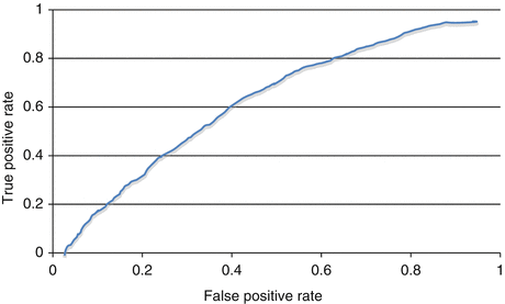
The model discrimination determines the ability to distinguish between both outcome events, e.g., survival or death. The model discrimination is calculated with the area under the receiver-operating-characteristic (ROC) curve and is measured by the c-statistic, which ranges from “0” to “1.” The ROC curve is plotted based on the true-positive and false-positive rates of the prediction of the outcome event, through multiple iterations of the model performance in the entire study population (Fig. 15.1). In this manner, a c-statistic of 0.5 has no discriminatory value because an event predicted as positive will be equally possible to be a true-positive or a false-positive event; thus, providing a predictive power not greater than random chance. A c-statistic of 0.7–0.9 is usually reported in most models with adequate predicted power (Bewick et al. 2004).


Fig. 15.1
Receiver-operating-characteristic curve. The c-statistic [range (0.0–1.0)] is calculated as the area under the receiver-operating-characteristic curve
15.2.4.3 Model Validation
It is preferable to validate the goodness of fit and discrimination in a different dataset than the one used to create the model. The original dataset can be partitioned into a training set (sample used to develop the model) and a testing set (sample used to validate the model). These categories are not required to be of the same size, but each one must be representative of the entire dataset. The validation process is conducted by applying the risk model into the testing set and recalculating the goodness of fit (p-value) and discrimination (c-statistic) (Bewick et al. 2005).
15.2.5 Methods for Risk-Adjusted Comparison of Outcomes
In order to determine areas in which to implement quality improvement measures, risk-adjusted methods are necessary in the comparison of institution-specific or surgeon-specific outcomes. The following are common indexes used for these comparisons:
15.2.5.1 Observed-to-Expected (O/E) Ratio
The observed and expected rates of an outcome event are calculated for a study population. The expected rate is calculated by averaging the predicted risk of the outcome event in each patient. A random effects variable may also be entered in the model to adjust for the random variation among institutions. The O/E ratio for a specific provider is compared to the O/E ratio of the entire population, which should be in very close proximity to the neutral value of 1.0. A significant difference in this comparison reflects a deviation of the outcome event for a particular provider.
Stay updated, free articles. Join our Telegram channel

Full access? Get Clinical Tree


