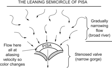
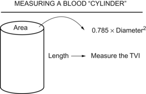
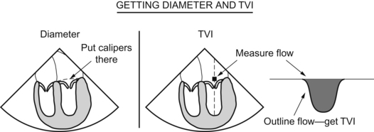
Here I think they’re driving at pulsed-wave Doppler versus continuous-wave Doppler. (It’s tough going through this and wondering “What are they thinking?”) To review, then, pulsed-wave Doppler takes a specific look at a specific velocity at a specific place. The pulse wave (PW) transducer is used as both a receiver and transmitter of ultrasound waves. A complete cycle of transmission waiting and receiving is called the pulse repetition frequency (PRF). The greater the depth of interrogation of the pulsed ultrasound beam the longer the waiting period. Therefore, the deeper the interrogation, the lower the PRF, and the lower the maximal velocity that can be measured. Pulsed-wave ultrasound is used to provide data for Doppler sonograms and color flow images.

Continuous-wave Doppler, in contrast, takes velocity measurements along the entire length of the beam, allowing you to measure high velocities, but not allowing you to know exactly where that measurement is made (also known as “range ambiguity”). In this modality, ultrasound is continually transmitted by one crystal and continually received by another.

Another thing they might be driving at here is PISA, the proximal iso velocity surface area.

This, too, is gone over ad nauseum in Chapter 3, but here goes. As blood flow converges toward a tight spot (Analogy? Think of a broad river coming to a narrow gorge), the flow will speed up. At a certain concentric area, the flow should all be at the same speed as the “chaos” of a broad river becomes the “organized tightness” of a narrow channel. This area will, when measured by color flow Doppler, hit the Nyquist limit and will start aliasing. Red flow will become blue, for example, in a semicircle. You can measure the area of this by the equation

This will come in handy as you do volume measurements and try to assess valve areas. At the risk of sounding like a broken record, go to the hemodynamic section to see these ideas put into action. (And into the kind of thing that would appear on an exam.)

This gets into the realm of the material in Chapter 3, the volume equations you use to measure valve areas, cardiac outputs, stroke volumes, and the like. The sample problems in that chapter illustrate better than this explanation, but here goes.

The main volume you will lug around through the heart is best thought of as a cylinder of blood. You will make various area measurements (area is 0.785 × diameter squared) and “length” measurements (the TVI, or time-velocity integral, which you get by outlining the flow through an area, and then the echo machine computer spits out a TVI, the integrated area under the flow curve).

A million times, you will make these measurements and apply them to get valve areas. Yeah, verily, I say unto you, do all the problems in the hemodynamics section and you will see what all of this means.

The gradient, or change in pressure, across a valve is measured by the Bernoulli equation:

The real Bernoulli equation is understood only by “brilliant French physicists at the turn of the 18th century”. You know, when all this stuff was figured out. Here are a few examples of Bernoulli’s equation in action:

Example 1: The velocity across a stenotic mitral valve is 4 meters/second. What is the gradient?

Note that the velocity has to be in meters/second to get a pressure in mmHg. Ask Bernoulli if you want to know why.

Example 2: The velocity going back across a regurgitant valve is 2 meters/second. What is the gradient?

Stay updated, free articles. Join our Telegram channel

Join