Quantification in Cardiac Magnetic Resonance Imaging and Computed Tomography
Rob J. van der Geest
Boudewijn P.F. Lelieveldt
Johan H.C. Reiber
Magnetic resonance imaging (MRI) and multislice computed tomography (MSCT) have become indispensable imaging modalities for evaluation of the cardiac system. MRI provides unique capabilities for studying many aspects of cardiac anatomy, function, perfusion, and viability in a single imaging session. Nevertheless, MSCT is rapidly gaining widespread clinical use for the evaluation of coronary anatomy and cardiac function. The recent technologic developments in MSCT have resulted in a tremendous improvement of image quality and high sensitivity and specificity for the detection of coronary stenosis.
Both MRI and MSCT are three-dimensional (3D) imaging modalities that are used for the evaluation of ventricular function. Volumetric measurement of the ventricular cavities and myocardium can be performed at high accuracy and precision as has been demonstrated in many experimental and clinical research studies. The 3D nature of these imaging modalities also provides detailed information of the cardiac system at a regional level. Among others, regional end-diastolic wall thickness and systolic wall thickening provide useful information for the assessment of the location, extent, and severity of ventricular abnormalities in ischemic heart disease. MRI can also be used to study blood flow and myocardial perfusion. Velocity-encoded cine MRI (VEC-MRI) is often used for the quantification of blood flow through the aortic and pulmonary valves and atrioventricular valve planes, which has shown to be clinically valuable in the evaluation of patients with complex congenital heart disease.
Typical cardiac MRI and MSCT examinations generate large data sets of images. To optimally and efficiently extract the relevant clinical information from these data sets, dedicated software solutions featuring automated image segmentation and optimal quantification and visualization methods are needed. Quantitative image analysis requires the definition of contours describing the inner and outer boundaries of the ventricles, which is a laborious and tedious task when based on manual contour tracing. Reliable automated or semiautomated image analysis software would be required to overcome these limitations. This chapter focuses on the
state-of-the-art postprocessing techniques for quantitative assessment of global and regional ventricular functions from cardiac MRI and MSCT.
state-of-the-art postprocessing techniques for quantitative assessment of global and regional ventricular functions from cardiac MRI and MSCT.
QUANTIFICATION OF VENTRICULAR DIMENSIONS AND GLOBAL FUNCTION
ACCURACY AND REPRODUCIBILITY OF VOLUMETRIC MEASUREMENTS FROM MULTISLICE SHORT-AXIS ACQUISITIONS
MRI and MSCT allow imaging of anatomic objects in multiple parallel sections, enabling volumetric measurements using the Simpson’s rule. According to Simpson’s rule, the volume of an object can be estimated by summation of the cross-sectional areas in each section multiplied by the section thickness. When there is a gap in between slices, this must be corrected for and the formula for volume becomes:
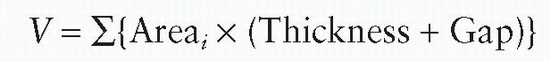
where V is the volume of the 3D object and Areai the area of the cross section in section number i.
The short-axis orientation is the most commonly applied image orientation for the assessment of left ventricular chamber size and mass. Although MRI is capable of directly acquiring images in any orientation, MSCT images are always generated in the axial orientation and image reformatting is required to obtain short-axis images. The short-axis orientation has advantages over other slice orientations because it yields cross-sectional slices almost perpendicular to the myocardium for the largest part of the left ventricle (LV). This results in minimal partial volume effect at the myocardial boundaries and subsequently provides optimal depiction of the myocardial boundaries. However, the curvature of the LV at the apical level leads to significant partial volume averaging. The image voxels in this area simultaneously intersect with blood and myocardium yielding indistinct myocardial boundaries. By minimizing the slice thickness, while keeping sufficient signal to noise, this partial volume effect at the apex can be reduced. Given the relatively small cross-sectional area of the LV in the apical section, the error introduced because of the partial volume effect will be minimal. However, partial volume averaging at the basal level of the heart has a much greater impact because at this level the cross-sectional area of the LV is largest. The base of the LV exhibits a through-plane motion in the apical direction during systole on the order of 1.3 cm (1,2). Therefore, the significance of partial volume varies over the cardiac cycle. Additional long-axis views may prove helpful in determining more accurately how a basal short-axis slice intersects with the various anatomic regions.
IMPACT OF SLICE THICKNESS AND SLICE GAP
It is a prerequisite for the accurate assessment of the ventricular volumes that the stack of short-axis slices covers the complete ventricle from base to apex. With MRI, a section thickness between 6 and 10 mm is used, and the gap between slices varies from no gap (consecutive slices) to 4 mm. With MSCT, any value can be chosen for the slice thickness and gap when generating a short-axis data set by reformatting the original images. Typical parameters for MSCT are a slice thickness between 4 and 8 mm usually without any intersection gap. Quantification of volumes and mass requires the definition of contours in the images describing the endocardial and epicardial boundaries of the myocardium in several phases of the cardiac cycle. Although an image voxel may contain several tissues, because of the partial volume effect, it is assumed that the traced contours represent the geometry of the ventricle at the center of the imaged section. As shown in Figure 6.1, the partial volume effect may lead to both over-and underestimation in the assessment of ventricular volume.
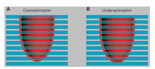 Figure 6.1. Left ventricular geometry intersected by multiple parallel short-axis sections. Given the same section thickness and intersection gap, both over- and underestimation of left ventricular volume can occur dependent on the position of the left ventricle (LV) with respect to the imaging slices. In situation (A) the most basal slice will be included in the volumetric assessment, whereas in (B), the most basal slice will not be taken into account because it intersects by less than 50% with the left ventricular myocardium. |
With a simple experiment using synthetically created left ventricular shapes and short-axis cross sections it can be shown how the partial volume problem may affect measurement accuracy and reproducibility. For this purpose a computer-generated average left ventricular geometry with a fixed size was constructed and short-axis cross sections were automatically derived while varying the position of the ventricular geometry along the long-axis direction. The shape used and its dimensions are presented in Figure 6.2. In this
experiment it is assumed that the contours in a short-axis slice will only be drawn in case more than 50% of the slice thickness intersects with myocardium. The results of the simulations as depicted in Figure 6.3 demonstrate that the measurement precision (or measurement variability) degrades with increasing distance between the slices. For typical imaging parameters (section thickness 6 mm, gap 4 mm) the measurement variability is between 4% and 5%. The measurement accuracy is not dependent on the slice thickness or slice gap used. A section thickness of 10 mm with no gap results in the same variability as a section thickness of 6 mm with a gap of 4 mm.
experiment it is assumed that the contours in a short-axis slice will only be drawn in case more than 50% of the slice thickness intersects with myocardium. The results of the simulations as depicted in Figure 6.3 demonstrate that the measurement precision (or measurement variability) degrades with increasing distance between the slices. For typical imaging parameters (section thickness 6 mm, gap 4 mm) the measurement variability is between 4% and 5%. The measurement accuracy is not dependent on the slice thickness or slice gap used. A section thickness of 10 mm with no gap results in the same variability as a section thickness of 6 mm with a gap of 4 mm.
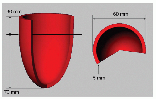 Figure 6.2. Left ventricular geometry used for the simulation experiments. The phantom consists of a half ellipsoid with a length of 70 mm and an outer diameter at the base of 60 mm; at the base the shape is extended with a cylinder with a diameter of 60 mm and a length of 30 mm. The thickness of the phantom was set to 5 mm. In the experiments the size of the object was varied between the dimensions shown and 80% of this size. |
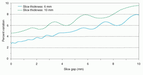 Figure 6.3. Results of volume calculation experiments using synthetically constructed left ventricular geometries. The variability of left ventricular volume estimates increases with increasing slice thickness and slice gap. For a setting of the imaging parameters, such as a thickness of 6 mm and a gap of 4 mm, the measurement variability is 5%. |
The result of this experiment has two important implications. First, variations between successive scans of the same patient may result in volumetric differences of up to 5%, which are inherent to the imaging technique used. Second, because the base of the heart has a significant through-plane motion component, the measurement variability of up to 5% will also be present over the cardiac cycle. Therefore, ejection fraction measurements will also be affected. By reducing the section thickness and the intersection gap, the variability in volumetric measurements can be reduced. For MSCT, in which short-axis reformats are derived from highresolution near-isotropic volumetric data, it is useful to use small values for the slice thickness without applying any gap.
GLOBAL FUNCTION ASSESSMENT USING RADIAL LONG-AXIS VIEWS
The accuracy of volumetric measurements from multislice short-axis acquisitions is mainly determined by the accurate identification of the most basal slice level and the accurate definition of the endocardial and epicardial contours in this slice level. However, because of the relatively large section thickness used, this is often difficult. The origin of the problem is the highly anisotropic nature of a typical short-axis examination in which the resolution in the Z-direction is much worse than the in-plane resolution. To overcome this limitation, Bloomer et al. (3) investigated the use of multiple radial long-axis views for quantification of left ventricular volumes and mass using a steady-state free precession (SSFP) MRI sequence. With a radial long-axis acquisition, multiple long-axis views are acquired sharing a common axis of rotation (the LV long-axis) at equiangular intervals. This orientation has intrinsic advantages over short-axis imaging because it allows clear visualization of the mitral and aortic valve planes. In addition, long-axis views have less partial volume effect near the apex. After definition of the ventricular contours, calculation of LV volume is performed by adding pie-shaped volume elements defined by the location of the axis of rotation, position of the contour, and angular interval between the image sections. Bloomer et al. demonstrated a good agreement between multislice short-axis and radial long-axis acquisitions. As a result of the improved visualization of the myocardial boundaries and definition of the base, interobserver agreement was better using the radial long-axis method. Figure 6.4 illustrates examples of magnetic resonance images acquired using radial long-axis orientation. It clearly shows that the definition of the base and the contrast between blood and myocardium are excellent. Further research is needed to evaluate whether radial longaxis acquisitions also prove to be valuable for the assessment of regional function.
MYOCARDIAL MASS
The measurement of heart muscle weight is of clinical importance to properly diagnose and understand a patient’s illness and condition, and to estimate the effects of treatment. To detect small changes in mass it is of paramount importance to use an accurate and reproducible measurement technique. Several validation studies have been performed comparing mass estimates as derived from MRI with postmortem mass measurements. In a study by Florentine et al. (4) a stack of axial slices was used to quantify left ventricular mass using the Simpson rule. In this early study, they found good agreement (r = 0.95, standard error of estimate = 13 g). Maddahi et al. (5) carried out extensive studies in a dog model comparing several slice orientations and measurement techniques for quantifying left ventricular mass. It was shown that in vivo estimates of left ventricular myocardial mass are
most accurate when the images are obtained in the shortaxis plane (r=0.98, standard error of estimate = 4.9 g).
most accurate when the images are obtained in the shortaxis plane (r=0.98, standard error of estimate = 4.9 g).
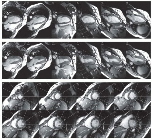 Figure 6.4. End-diastolic (top) and end-systolic (middle) magnetic resonance images acquired in radial long-axis views using steady-state free precession (SSFP) magnetic resonance imaging (MRI). Note the excellent conspicuity of the LV myocardial wall from base to apex. Orientation of the radial long-axis views (white lines in short-axis images, bottom). (Image data courtesy of M. Friedrich.) |
LEFT VENTRICULAR MASS
For the LV it is generally believed and also supported by literature that the short-axis orientation is the most appropriate imaging plane. To obtain optimal accuracy and reproducibility it is important to cover the complete ventricle from apex to base with a sufficient number of slices. Quantification of mass requires the definition of contours in the images describing the endocardial and epicardial boundaries in the stack of images. The muscle volume is assessed from these contours by applying Simpson’s rule. The myocardial mass is derived by multiplying the muscle volume with the specific density of myocardium (1.05 g/cm3).
Typically, a section thickness between 6 and 10 mm is used with an intersection gap between 0 and 4 mm. At the apex and basal sections significant partial volume averaging will occur because of the section thickness used and tracing of the myocardial boundaries may not be trivial. Similarly, partial volume averaging will cause significant difficulties in interpreting sections with a highly trabeculated myocardial wall and papillary muscles (6). There is no general consensus
on whether to include or exclude papillary muscles and trabeculae in the left ventricular mass. Although it is evident that inclusion of these structures would result in more accurate myocardial mass measurements, for regional wall thickening analysis it is important to exclude these structures to avoid artifacts in the quantification. Whether to use an enddiastolic or end-systolic time frame for the measurement is also a subject of ongoing debate. Most likely, optimal accuracy and reproducibility are obtained by averaging multiple time frames, but this will have practical objections in case the contours are derived by manual tracing.
on whether to include or exclude papillary muscles and trabeculae in the left ventricular mass. Although it is evident that inclusion of these structures would result in more accurate myocardial mass measurements, for regional wall thickening analysis it is important to exclude these structures to avoid artifacts in the quantification. Whether to use an enddiastolic or end-systolic time frame for the measurement is also a subject of ongoing debate. Most likely, optimal accuracy and reproducibility are obtained by averaging multiple time frames, but this will have practical objections in case the contours are derived by manual tracing.
RIGHT VENTRICULAR MASS
For the right ventricle (RV) and geometrically abnormally shaped LVs, multiple sections are required for an accurate volume assessment (7). MRI experiments with different slice orientations in phantoms and ventricular casts have shown that no significant difference can be observed in accuracy and reproducibility between slice orientations (8). However, in a clinical situation the choice of slice orientation also depends on the availability of a clear depiction of anatomic features that are needed to define the myocardial boundaries. Volumetric quantification of the RV may be better performed on the basis of axial views (9). This view shows improved anatomic detail and allows better differentiation between the right ventricular and atrial lumen. Nevertheless, for practical reasons, the right ventricular mass is often measured using a stack of short-axis slices, which is also used for measuring the left ventricular dimensions.
QUANTIFICATION OF VENTRICULAR VOLUMES AND GLOBAL FUNCTION
Assessment of global ventricular function requires volumetric measurement of the ventricular cavities in at least two points in the cardiac cycle: The end-diastolic and end-systolic phases. A vast amount of reports describe the applicability of MRI for accurate and reproducible quantification of left and right ventricular volumes using various MRI strategies (4,10). Cardiac-gated MSCT also allows quantification of global function (11). Sufficient temporal resolution is required to properly capture the end-systolic phase. Generally a temporal resolution, or phase interval, on the order of 40 to 50 ms is assumed to be sufficient. Although MRI can provide such temporal resolution, the temporal resolution of MSCT does not yet fulfill this requirement. However, global function results obtained by MSCT are in good agreement with results derived from MRI (12,13). For geometrically normal LVs, one could rely on geometric models to derive the volumes from one or two long-axis imaging sections. In a group of 10 patients with LV hypertrophy and 10 healthy subjects, Dulce et al. (14) demonstrated a good agreement between biplane volumetric measurements using either the modified Simpson’s rule of an ellipsoid model or true 3D volumetric measurements using a multislice MRI approach. In another study by Chuang et al. (15), 25 patients with dilated cardiomyopathies were evaluated using both biplane and 3D multislice approach. They reported a poor correlation between the two measurement methods. At the present state, a single section with sufficient temporal resolution can be acquired within a single breath-hold on most available MRI systems. The total duration of acquiring the 8 to 12 sections required to image the entire ventricular cavity is on the order of 5 minutes (16,17). All sections should be acquired at the same end-expiration or end-inspiration phase; otherwise reliable 3D quantification of volumes from the obtained images is not possible. In MSCT, the complete volumetric data set is acquired during a single breath-hold of 10 to 30 seconds.
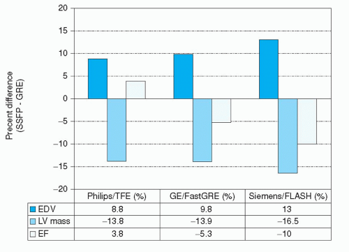 Figure 6.5. Comparison of LV dimensions measured with an SSFP sequence or segmented gradientecho technique. (Data derived from: Alfakih K, Plein S, Thiele H, et al. Normal human left and right ventricular dimensions for MRI as assessed by turbo gradient echo and steady-state free precession imaging sequences. J Magn Reson Imaging. 2003;17(3):323-329; Lee VS, Resnick D, Bundy JM, et al. Cardiac function: MR evaluation in one breath-hold with real-time True Fisp imaging with steady-state precession. Radiology. 2002;222:835-842; and Wei LI, Stern JS, Mai VM, et al. MR assessment of left ventricular function: Quantitative comparison of fast imaging employing steady-state acquisition (FIESTA) with fast gradient echo cine technique. J Magn Reson Imaging. 2002;16(5):559-564.) |
Quantitative analysis starts with manual or (semi-) automated segmentation of the myocardium and blood pool in the images. Once contours have been defined in the stack of images describing the endocardial and epicardial boundaries of the myocardium, volumetric measurements including stroke volume and ejection fraction can be obtained by
applying Simpson’s rule. Normal values for global ventricular function and mass have been reported by several investigators for different populations and pulse sequences (18,19 and 20). It is important to note that normal values obtained using the newer SSFP-type sequences differ significantly from values obtained with previous techniques. The improved contrast between blood and myocardium in SSFP is associated with larger end-diastolic and end-systolic cavity volumes, smaller wall thickness values, and lower LV mass (20,21 and 22). In direct comparisons of SSFP with conventional fast gradient-echo techniques within the same individuals, differences in LV mass of up to 16.5% were reported (Fig. 6.5).
applying Simpson’s rule. Normal values for global ventricular function and mass have been reported by several investigators for different populations and pulse sequences (18,19 and 20). It is important to note that normal values obtained using the newer SSFP-type sequences differ significantly from values obtained with previous techniques. The improved contrast between blood and myocardium in SSFP is associated with larger end-diastolic and end-systolic cavity volumes, smaller wall thickness values, and lower LV mass (20,21 and 22). In direct comparisons of SSFP with conventional fast gradient-echo techniques within the same individuals, differences in LV mass of up to 16.5% were reported (Fig. 6.5).
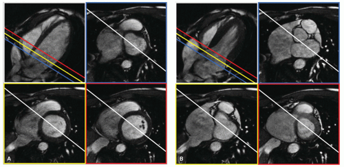 Figure 6.6. Four-chamber long-axis view and three basal level short-axis views acquired within the same examination. Short-axis and long-axis imaging planes intersect with each other (white lines indicate intersection of long-axis view with short-axis slices; colored lines indicate intersection of the three short-axis slices with the long-axis image). The movement of the base toward the apex in systole can easily be appreciated. Review of how long-axis and short-axis planes intersect may facilitate the interpretation of basal level shortaxis images and may be valuable during tracing of the contours. |
At the basal imaging sections, a clear visual separation between the LV and the left atrium is often absent because the imaging section may contain both ventricular and atrial cavity and muscle. It is important to realize that while the imaging sections are fixed in space, the left ventricular annulus exhibits a motion in the apical direction on the order of 1.3 cm in normal hearts (1). Consequently, myocardium that is readily visible in an end-diastolic time frame may be replaced by left ventricular atrium in the end-systolic time frame. Additional long-axis views may be helpful to more reliably analyze the most basal and apical slice levels of a multislice short-axis study (2). Figure 6.6 displays enddiastolic and end-systolic time frames in a long-axis view and three basal short-axis sections obtained during a single MRI examination. The lines, indicating the intersections of the imaging planes, provide helpful additional information for interpreting the structures seen in the short-axis images.
QUANTIFICATION OF REGIONAL WALL MOTION AND WALL THICKENING USING THE CENTERLINE METHOD FROM DYNAMIC SHORT-AXIS IMAGES
The excellent depiction of the endocardial and epicardial boundaries of the left ventricular myocardium forms the basis of quantitative analysis of regional myocardial function. Quantitative analysis methods for endocardial wall motion are hampered by the presence of rigid body motion of the heart. A floating centroid, based on the center of gravity of the endocardial or epicardial contours, can be used to isolate the rigid body motion from the actual endocardial deformation. On the other hand, quantification of wall thickness and thickening does not have this disadvantage. It has been demonstrated that wall-thickening analysis is more sensitive in the detection of dysfunctional myocardium than wall-motion analysis (23,24). The optimal slice orientation for wall-thickness analysis of the LV is the short-axis plane because in this orientation the major part of the myocardial wall is perpendicular to the imaging section (25,26,27 and 28


Stay updated, free articles. Join our Telegram channel
Full access? Get Clinical Tree
