, Chandan Karmakar3, Michael Brennan3, Andreas Voss4 and Marimuthu Palaniswami3
(1)
Department of Biomedical Engineering, Khalifa University, Abu Dhabi, UAE
(2)
Department of Electrical and Electronic Engineering, The University of Melbourne, Melbourne, VIC, Australia
(3)
Electrical and Electronic Engineering, The University of Melbourne, Melbourne, VIC, Australia
(4)
Department of Medical Engineering and Biotechnology, University of Applied Sciences Jena, Jena, Germany
Abstract
In this chapter, we present new results in developing a novel mathematical model that describes the interactions between the sympathetic and the parasympathetic nervous systems and heart rate fluctuations over a short-term period of 5–10 min. While our model is based upon well-accepted physiological principles, the mathematical formulation permits in-depth numerical and analytical investigations yielding valuable insight into clinical RR interval analysis techniques.
3.1 Introduction
In this chapter, we present new results in developing a novel mathematical model that describes the interactions between the sympathetic and the parasympathetic nervous systems and heart rate fluctuations over a short-term period of 5–10 min. While our model is based upon well-accepted physiological principles, the mathematical formulation permits in-depth numerical and analytical investigations yielding valuable insight into clinical RR interval analysis techniques.
Standard analysis techniques commonly estimate the levels of sympathetic and parasympathetic activity from the variability in the RR intervals. Our attention has focused on two specific HRV analysis techniques. The first is the frequency-domain spectral analysis of RR intervals [14, 101, 119–121]. RR interval Poincaré plot analysis is the second technique [59, 87, 89, 91, 94]. The main objective of our model is to provide insight into the significance of Poincaré plot morphology, not to accurately reproduce the complex autonomic activity of any particular individual.
Our model emulates the differing varieties of Poincaré plot patterns seen in subjects over a range of sympathovagal balances. In addition, the model provides a unique link between spectral analysis techniques and the emerging analysis techniques that rely on the shape and/or other morphological properties of the Poincaré plot. Analytical results on the “lengths” and “widths” of the Poincaré plots generated by our model are developed. Simulations are employed to confirm the analytical results on the model. In order to evaluate the validity and scope of the model and analysis we provide results using a set of data from actual subjects.
3.2 Autonomous Nervous System and HRV Analysis
It is well known that perturbations to autonomic activity, such as respiratory sinus arrhythmia and vasomotor oscillations, cause corresponding fluctuations in heart rate [8, 102]. HRV analysis seeks to determine the autonomic activity from heart rate variability. Spectral analysis is the standard technique used to determine the presence of respiratory sinus arrhythmia and vasomotor oscillations [8, 122]. This is accomplished by dividing the spectrum into low-(0.04–0.15 Hz) and high-(0.15–0.4 Hz) frequency bands, known as the LF and HF bands, effectively distinguishing between rapid respiratory modulator activity and slow vasomotor modulation of heart rate (see Fig. 3.1a). HF power is supposedly a pure measure of parasympathetic activity, and LF power is reflective of sympathetic modulation and parasympathetic tone, although it is sometimes considered to reflect sympathetic tone [120]. In this chapter, spectral estimates are given by the autoregressive (AR) parametric technique using the modified covariance method [123] for the smooth spectrum and easy identification of the spectral peaks.
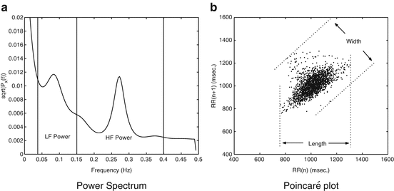

Fig. 3.1
Plot (a) is the HRV spectrum. The respiratory component near 0.3 Hz and the vasomotor component near 0.1 Hz are clearly present. Plot (b) is the Poincaré plot of the same data. The length and the width are shown graphically on the plot. Figure adapted from Brennan et al. [118]
The Poincaré plot is a scatter plot of the current RR interval plotted against the preceding RR interval. Poincaré plot analysis is a quantitative visual technique, whereby the shape of the plot is categorized into functional classes [59, 91]. The plot provides summary information as well as detailed beat-to-beat information on the behaviour of the heart [94]. Points above the line of identity indicate RR intervals that are longer than the preceding RR interval, and points below the line of identity indicate a shorter RR interval than the previous. Accordingly, the dispersion of points perpendicular to the line of identity (the “width”) reflects the level of short-term variability. This dispersion can be quantified by the standard deviation of the distances the points lie from the line of identity. This measure is equivalent to the standard deviation of the successive differences of the RR intervals (SDSD or RMSSD) [89]. The standard deviation of points along the line of identity (the “length”) reflects the standard deviation of the RR intervals (SDNN). Figure 3.1b details these quantitative measures of Poincaré plot shape. Poincaré plots appear under different names in the literature: scatter plots, first return maps and Lorenz plots being prominent terms. A distinct advantage of Poincaré plots is their ability to identify beat-to-beat cycles and patterns in data that are difficult to identify with spectral analysis [59, 91].
3.3 Physiological HRV Model
In this section we develop a model using a coupled network of oscillators, each representing a specific characteristic or facet of the baroreflex and autonomic nervous system. The architecture of the network and the coupling are shown in Fig. 3.2. The coupling constants C s and C p denote the level at which the corresponding oscillator modulates the sinus node oscillator. For the purpose of clarity, we define the respiratory oscillator as the parasympathetic oscillator.
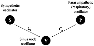

Fig. 3.2
Three coupled oscillators representing the cardiac control system. Figure adapted from Brennan et al. [118]
3.3.1 Sympathetic Oscillator
The sympathetic oscillator (S) is governed by Eq. 3.1:

where s represents the level of sympathetic activation. Sympathetic activity occurs on a slow time scale, i.e. it reacts slowly, altering heart rate over a long duration [8, 101, 124]. Accordingly it is assigned a small value, producing slow waves of approximately 10–15 s duration. This oscillator represents the combined low-frequency (LF) power of the HRV spectrum, which includes vasomotor activity. It is generally accepted that low levels of sympathetic activity will result in slow oscillations of sympathetic nerve activity entrained to the vasomotor oscillations.

(3.1)
As the level of sympathetic activity increases, these oscillations are damped and the fluctuations disappear such that under intense sympathetic drive the heart rate becomes metronomic in its regularity. This damped effect can be achieved by taking ω s → 0 or by reducing the coupling between the sympathetic oscillator and the sinus oscillator by taking C s → 0.
3.3.2 Parasympathetic Respiratory Oscillator
Respiratory oscillations affect both the sympathetic and parasympathetic nervous systems. However, because of the slow response time of the sympathetic system, these rapid oscillations, often in the order of 2–3 seconds per cycle, are mediated purely by the parasympathetic system [8, 101, 124]. The effects of respiration are described by the parasympathetic respiratory oscillator (P), which is governed by Eq. 3.2:

where p represents the level of parasympathetic respiratory activation. As the parasympathetic system typically reacts faster than the sympathetic system, but altering heart rate over a much shorter duration, this oscillator has a value of ω p larger than ω s . Values in the simulation produce oscillations of duration between 2 and 5 s. This oscillator is intended to represent short-term activity impinging on the sinus node via the parasympathetic nervous system.

(3.2)
3.3.3 Sinus Oscillator
The sinus node oscillator is based on the formulation of the well-known integral pulse frequency modulation (IPFM) model. Hyndman and Mohn first suggested the IPFM model as a representation of the cardiac pacemaker and the suitability for modeling the sinus node has been discussed by a number of researchers in the area of point event processes [97, 99, 102]. The IPFM model is a useful description of how cardiac events are modulated by autonomic nervous activity and has had numerous applications in describing the generation of point event processes [99, 102]. The IPFM model generates heartbeats by integrating an input signal until it reaches a preset threshold of unity. At this point a pulse is produced and the integrator is reset to zero. See Fig. 3.3. The mathematical representation is given in Eq. 3.3:
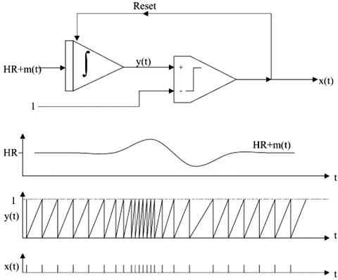

Fig. 3.3
IPFM model. The input signal H R + m(t) is integrated until the integrator output y(t) reaches the threshold of unity. At this point a pulse is produced in the output signal x(t) and the integrator is reset. Figure adapted from Brennan et al. [118]

(3.3)
The signal m(t) is the input signal representing autonomic activity and t k is the time of the k t h R wave. When the input signal is zero the IPFM model generates heartbeats with an interval equal to  where H R is a variable parameter which represents mean heart rate. It is equal to the actual frequency of heartbeats in the absence of any modulatory autonomic nervous activity. The input signal m(t) represents the effects of modulatory autonomic nervous input and is defined by Eq. 3.4. If the input signal is positive then heartbeats are generated at a faster rate while a negative input signal causes heartbeats to be generated at a slower rate. The function x(t) represents the series of pulses representing the heartbeats generated by the model while y(t) designates the integrator’s output as a function of time.
 where H R is a variable parameter which represents mean heart rate. It is equal to the actual frequency of heartbeats in the absence of any modulatory autonomic nervous activity. The input signal m(t) represents the effects of modulatory autonomic nervous input and is defined by Eq. 3.4. If the input signal is positive then heartbeats are generated at a faster rate while a negative input signal causes heartbeats to be generated at a slower rate. The function x(t) represents the series of pulses representing the heartbeats generated by the model while y(t) designates the integrator’s output as a function of time.
We have formulated the modulation of the sinus oscillator by the sympathetic and parasympathetic oscillators as described by Eq. 3.4:


(3.4)
As a result, the sinus oscillator beats at a base rate of H R Hertz, which is increased or decreased in an additive linear fashion by sympathetic and parasympathetic respiratory modulation. For the modulating frequencies to appear unaliased in the beat sequence, the mean beat frequency H R should be higher than the highest modulating frequency component, ω p :
![$$\displaystyle{ HR \gg \frac{\omega _{p}} {2\pi }> \frac{\omega _{s}} {2\pi } }$$
” src=”/wp-content/uploads/2017/01/A273083_1_En_3_Chapter_Equ5.gif”></DIV></DIV><br />
<DIV class=EquationNumber>(3.5)</DIV></DIV></DIV><br />
<DIV class=Para>The coupling constants <SPAN class=EmphasisTypeItalic>C</SPAN> <SUB><SPAN class=EmphasisTypeItalic>s</SPAN> </SUB>and <SPAN class=EmphasisTypeItalic>C</SPAN> <SUB><SPAN class=EmphasisTypeItalic>p</SPAN> </SUB>reflect the levels of sympathetic and parasympathetic <SPAN class=EmphasisTypeItalic>modulation</SPAN> of the sinus node, which is not equivalent to the tonic (mean) levels of sympathetic and parasympathetic activity. The tonic autonomic influences are included in the parameter <SPAN class=EmphasisTypeItalic>H R</SPAN> which is a combined function of sympathetic and parasympathetic activity, hormonal responses and various parameters of the individual such as blood pressure. Accordingly <SPAN class=EmphasisTypeItalic>H R</SPAN> is a function of the intrinsic heart rate <SPAN class=EmphasisTypeItalic>H R</SPAN> <SUB>0</SUB> and the tonic influences of the autonomic system commonly referred to as the sympathovagal balance [<CITE><A href=]() 125]. While the exact nature of sympathovagal balance is not completely understood, this concept has been formalized by the following model,
125]. While the exact nature of sympathovagal balance is not completely understood, this concept has been formalized by the following model,  , due to Rosenblueth and Simeone [124] and Katona et al. [126] in which m > 1 is the net sympathetic influence and n < 1 is the net parasympathetic influence. It is still being debated if there exist any reliable connections between the tonic influences m and n and the levels of modulation C s and C p ; however, it is often observed that heart rate and HRV are inversely related.


 , due to Rosenblueth and Simeone [124] and Katona et al. [126] in which m > 1 is the net sympathetic influence and n < 1 is the net parasympathetic influence. It is still being debated if there exist any reliable connections between the tonic influences m and n and the levels of modulation C s and C p ; however, it is often observed that heart rate and HRV are inversely related.
Accordingly, we model H R as a free variable which is not determined explicitly by C s or C p . In other words, our model characterizes nervous activity as separate modulatory and static effects. C s and C p should be chosen such that H R + m(t) is strictly positive. Choosing C s + C p < H R guarantees this.
3.4 Mathematical Analysis of HRV Model Using Poincaré Plot
This section develops a mathematical analysis used to investigate the length and width of the Poincaré plots generated from the HRV model developed in the previous sections. As the model is a simplification of actual HRV mechanisms these results will not apply to real HRV data in an exact sense. However, the results provide clear insight into the manner in which Poincaré plot descriptors vary as sympathetic and parasympathetic modulation levels are varied. Specifically, we characterize the theoretical dependency between low- and high-frequency modulators and the shape of an RR interval Poincaré plot generated by our model.
In accomplishing this analysis we require an explicit solution to the RR interval series. The remainder of this section derives this result. By defining the time of the initial beat to be the origin t 0 = 0, the defining equation for the IPFM oscillator (Eq. 3.3) can be expressed non-recursively as
![$$\displaystyle{ \int _{0}^{t_{k} }[HR + m(t)]\mathrm{d}t = k }$$](/wp-content/uploads/2017/01/A273083_1_En_3_Chapter_Equ6.gif)
where m(t) is the modulating signal. In our model m(t) consists of two frequency components. It turns out to be just as easy to work with N frequency components, so we consider  with
with  for all n, i.e. slow modulation. The defining equation becomes
![$$\displaystyle{ \int _{0}^{t_{k} }[1 + \overline{I}\sum _{n=1}^{N}C_{ n}\cos (\omega _{n}t +\phi _{n})]\mathrm{d}t = k\overline{I} }$$](/wp-content/uploads/2017/01/A273083_1_En_3_Chapter_Equ7.gif)
![$$\displaystyle{ \int _{0}^{t_{k} }[HR + m(t)]\mathrm{d}t = k }$$](/wp-content/uploads/2017/01/A273083_1_En_3_Chapter_Equ6.gif)
(3.6)
 with
with  for all n, i.e. slow modulation. The defining equation becomes
![$$\displaystyle{ \int _{0}^{t_{k} }[1 + \overline{I}\sum _{n=1}^{N}C_{ n}\cos (\omega _{n}t +\phi _{n})]\mathrm{d}t = k\overline{I} }$$](/wp-content/uploads/2017/01/A273083_1_En_3_Chapter_Equ7.gif)
(3.7)
We have also divided through by H R and expressed  to make the equations simpler. After integrating, the general relationship

is obtained. Performing the substitution  , as per De Boer et al. [99], the following nonlinear relationship for δ k is obtained:

 to make the equations simpler. After integrating, the general relationship
(3.8)
 , as per De Boer et al. [99], the following nonlinear relationship for δ k is obtained:
(3.9)
The δ k terms represent the amount each beat deviates from the regular pulse train  . Equation 3.9 can be linearized about δ k = 0 provided ω n δ k is small for all
 ![$$n\varepsilon [1..N]$$](/wp-content/uploads/2017/01/A273083_1_En_3_Chapter_IEq8.gif) . If the event times are close to a regular pulse train (
. If the event times are close to a regular pulse train ( ) and the modulation frequencies are less than the mean beat frequency (ω n < 2π H R) it is obvious that
  . Hence for a large class of practical pulse trains, including RR intervals, a linear analysis is an accurate approximation. Linearizing about δ k = 0 we obtain

 . Equation 3.9 can be linearized about δ k = 0 provided ω n δ k is small for all
 ![$$n\varepsilon [1..N]$$](/wp-content/uploads/2017/01/A273083_1_En_3_Chapter_IEq8.gif) . If the event times are close to a regular pulse train (
. If the event times are close to a regular pulse train ( ) and the modulation frequencies are less than the mean beat frequency (ω n < 2π H R) it is obvious that
  . Hence for a large class of practical pulse trains, including RR intervals, a linear analysis is an accurate approximation. Linearizing about δ k = 0 we obtain
(3.10)
Solving for δ k gives the final expression for the beat times:

(3.11)
The RR intervals are  . For our model, N = 2 and C 1 = C s , C 2 = C p , ω 1 = ω s , ω 2 = ω p and
  . In this case, Eq. 3.11 provides us with an accurate approximation to the RR interval series generated by our HRV model. This result holds so long as the intervals are approximately regular and the modulation is slow. This is generally the case for RR intervals. However, for subjects with very large HRV the assumption that the intervals are approximately regular may be somewhat inaccurate. For the assumption
  to be compromised, an RR interval would have to deviate from the mean RR interval by an amount
  greater than
  .
.
 . For our model, N = 2 and C 1 = C s , C 2 = C p , ω 1 = ω s , ω 2 = ω p and
  . In this case, Eq. 3.11 provides us with an accurate approximation to the RR interval series generated by our HRV model. This result holds so long as the intervals are approximately regular and the modulation is slow. This is generally the case for RR intervals. However, for subjects with very large HRV the assumption that the intervals are approximately regular may be somewhat inaccurate. For the assumption
  to be compromised, an RR interval would have to deviate from the mean RR interval by an amount
  greater than
  .
.Stay updated, free articles. Join our Telegram channel

Full access? Get Clinical Tree


