, Chandan Karmakar3, Michael Brennan3, Andreas Voss4 and Marimuthu Palaniswami3
(1)
Department of Biomedical Engineering, Khalifa University, Abu Dhabi, UAE
(2)
Department of Electrical and Electronic Engineering, The University of Melbourne, Melbourne, VIC, Australia
(3)
Electrical and Electronic Engineering, The University of Melbourne, Melbourne, VIC, Australia
(4)
Department of Medical Engineering and Biotechnology, University of Applied Sciences Jena, Jena, Germany
Abstract
The method and importance of capturing temporal variation using standard descriptors (SD1 and SD2) of Poincaré plot have been presented in Chap. 2. However, this does not include the temporal variation at point-to-point level of the plot. In addition, SD1 and SD2 descriptors are linear statistics (Brennan et al., IEEE Trans. Biomed. Eng. 48:1342–1347, 2001) and hence the measures do not directly quantify the nonlinear temporal variations in the time series contained in the Poincaré plot. Although SD1/SD2 is considered as a nonlinear measure, it yields mixed results when applied to the data sets that form multiple clusters in a Poincaré plot due to complex dynamic behaviours (Brennan et al., IEEE Trans. Biomed. Eng. 48:1342–1347, 2001). This is because the technique relies on the existence of a single cluster or a defined pattern (Christopher et al., Biophys. J. 82:206–214, 2002; Schechtman et al., Pediatr. Res. 40:571–577, 1996). Therefore, further studies are required in defining new descriptors for analysing temporal variability of time series using Poincaré plots. Another driving force behind this study is the fact that the visual pattern of the Poincaré plot of heart rate variability signals relies upon clinical scenarios and the application of the existing standard descriptors in various studies has resulted in limited success.
4.1 Introduction
The method and importance of capturing temporal variation using standard descriptors (SD1 and SD2) of Poincaré plot have been presented in Chap. 2. However, this does not include the temporal variation at point-to-point level of the plot. In addition, SD1 and SD2 descriptors are linear statistics [112] and hence the measures do not directly quantify the nonlinear temporal variations in the time series contained in the Poincaré plot. Although SD1/SD2 is considered as a nonlinear measure, it yields mixed results when applied to the data sets that form multiple clusters in a Poincaré plot due to complex dynamic behaviours [112]. This is because the technique relies on the existence of a single cluster or a defined pattern [128, 129]. Therefore, further studies are required in defining new descriptors for analysing temporal variability of time series using Poincaré plots. Another driving force behind this study is the fact that the visual pattern of the Poincaré plot of heart rate variability signals relies upon clinical scenarios and the application of the existing standard descriptors in various studies has resulted in limited success.
The inherent assumption behind using consecutive RR points in Poincaré plot is that the “present-RR-interval” significantly influences the “following-RR-interval”. Various researchers reported that varying lags of Poincaré plot give better understanding about the autonomic control of the heart rate that influence the short-term and long-term variability of the heart rate [57, 91]. A system can have different short-and long-term correlations on different time scales. When the sampling interval is less than the short-time correlation length, then these short-time correlations can be predominantly seen [130]. So in the context of short- or long-term variability, any point can influence at least a few successive points. Lerma et al. [131] reported that the current RR interval can influence up to approximately eight subsequent RR intervals in the context of the short-term variability. In another study, Thakre and Smith examined the theoretical demand with different lags and showed that there is a curvilinear relationship between lag Poincaré plot indices for normal subjects, which is lost in congestive heart failure (CHF) patients [132]. The relation between lags and width of Poincaré plot (SD1) has been reported by Goshvarpour et al. [133]. Therefore, measurement from a series of lagged Poincaré plots (multiple lag correlation) can potentially provide more information about the behaviour of the underlying system than the conventional lag-1 plot measurements [131].
The hypothesis of this chapter is that any descriptor that captures temporal information and is a function of multiple lag correlation, would provide more insight into the system rather than conventional measurements of variability of Poincaré plot (SD1 and SD2), which are parameters of a lag-1 correlation. In order to test this hypothesis, we propose a novel descriptor, complex correlation measure (CCM), for Poincaré plot that can be applied to measure the temporal variation of the Poincaré plot and is a function of multiple lag correlation of the signal.
4.2 Nonlinear Dynamics
4.3 Limitation of Standard Descriptors of Poincaré Plot
SD1 and SD2 represent the distribution of the signal in 2D space and carry only spatial (shape) information. It should be noted that many possible RR interval series result in identical plot with exactly similar SD1 and SD2 values irrespective of different temporal structures. For example, two signals with similar SD1 and SD2 values, top panels (Fig. 4.1), are different in terms of temporal structure, bottom panels (Fig. 4.1).
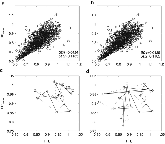

Fig. 4.1
Two different time series of length N (N = 1, 000) with similar SD1 and SD2 values are shown (m = 2) on top panel (a and b). In the bottom panel (c and d) the underlying dynamics of first 20 points of both time series are shown to be different
Lerma et al. have shown that the measurement from a multiple lag Poincaré plot provides more information than any measure from single lag Poincaré plot [131]. Indeed, the Poincaré plot at any lag-m is more of a generalized scenario, where other levels of temporal variation of the dynamic system are hidden. As shown in equation sets 2.14 and 2.15, for any m, the descriptors SD1 and SD2 only indicate m lag correlation information of the plot. This essentially conveys overall behaviour of the system neglecting its detail temporal variation. The Poincaré plot of RR interval time series for three different lags is shown in Fig. 4.2. From the plots, it is obvious that for any time-series signal, different lag plots better reveal the behaviour of the signal than the single lag plot. The CCM is not only related to the SD1 and SD2, but it also provides temporal information, which can be used to quantify the temporal dynamics of the system.
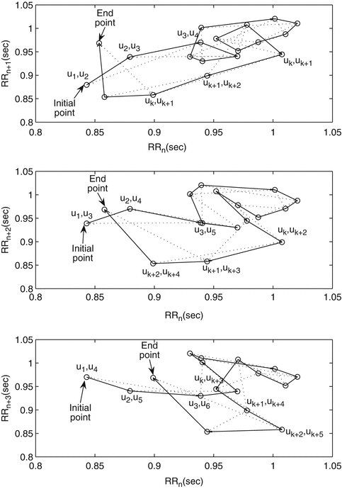

Fig. 4.2
Sequence of points (R R n , R R n + τ ) plotted and the triangle formed by each consecutive three points. Here,  and
and  .
.
 and
and  .
.4.4 Complex Correlation Measures in Poincaré Plot: A Novel Nonlinear Descriptor
The proposed descriptor CCM is computed using a moving window which embeds the temporal information of the signal. This moving window is comprised of three consecutive points from the Poincaré plot and the area of the triangle formed by these three points is computed. This area measures the temporal variation of the points in the window. If three points are aligned on a line then the area is zero, which represents the linear alignment of the points. Moreover, since the individual measure involves three points of the two-dimensional plot, it is comprised of at least four different points of the time series for lag m = 1 and at most six points in case of lag m ≥ 3. Hence the measure conveys information about four different lag correlations of the signal. Now, suppose the ith moving window is comprised of points a(x1, y1), b(x2, y2) and c(x3, y3) then the area of the triangle (A) for ith window can be computed using the following determinant:

where A is defined on the real line ℜ and


(4.1)

If Poincaré plot is composed of N points then the temporal variation of the plot, termed as CCM, is composed of all overlapping three point windows and can be calculated as

where m represents lag of Poincaré plot and C n is the normalizing constant which is defined as  and represents the area of the fitted ellipse over Poincaré plot. The lengths of major and minor axis of the ellipse are 2SD1 and 2SD2.

(4.2)
 and represents the area of the fitted ellipse over Poincaré plot. The lengths of major and minor axis of the ellipse are 2SD1 and 2SD2.
Let the RR time series be composed of N RR interval values and defined as  . As shown in Fig. 4.2, the lag-1 Poincaré plot consists of N − 1 numbers of 2D set of points P P, where
  can be represented by
  and similarly for lag of m, N − m numbers of 2D points are expressed as
 Hence, for lag-m Poincaré plot, the first window will be composed of points
  and from Eq. 4.1, the area A can be calculated as
![$$\displaystyle\begin{array}{rcl} A(1)& =& \frac{1} {2}[u_{1}u_{2+m} - u_{1}u_{3+m} + u_{3}u_{1+m} - u_{2}u_{1+m} + u_{2}u_{3+m} - u_{3}u_{2+m}].{}\end{array}$$](/wp-content/uploads/2017/01/A273083_1_En_4_Chapter_Equ3.gif)
 . As shown in Fig. 4.2, the lag-1 Poincaré plot consists of N − 1 numbers of 2D set of points P P, where
  can be represented by
  and similarly for lag of m, N − m numbers of 2D points are expressed as
 and from Eq. 4.1, the area A can be calculated as
![$$\displaystyle\begin{array}{rcl} A(1)& =& \frac{1} {2}[u_{1}u_{2+m} - u_{1}u_{3+m} + u_{3}u_{1+m} - u_{2}u_{1+m} + u_{2}u_{3+m} - u_{3}u_{2+m}].{}\end{array}$$](/wp-content/uploads/2017/01/A273083_1_En_4_Chapter_Equ3.gif)
(4.3)
Similarly the second and  th window is composed of points
 and
and  respectively. Hence, the area, A, for second and
  th window can be calculated as
![$$\displaystyle\begin{array}{rcl} A(2)& =& \frac{1} {2}[u_{2}u_{3+m} - u_{2}u_{4+m} + u_{4}u_{2+m} - u_{3}u_{2+m} \\ & & +u_{3}u_{4+m} - u_{4}u_{3+m}] {}\end{array}$$](/wp-content/uploads/2017/01/A273083_1_En_4_Chapter_Equ4.gif)
![$$\displaystyle\begin{array}{rcl} A(N - m - 2)& =& \frac{1} {2}[u_{N-m-2}u_{N-1} - u_{N-m-2}u_{N} + u_{N-m}u_{N-2} \\ & & -u_{N-m-1}u_{N-2} + u_{N-m-1}u_{N} - u_{N-m}u_{N-1}].{}\end{array}$$](/wp-content/uploads/2017/01/A273083_1_En_4_Chapter_Equ5.gif)
Using Eqs. 4.2–4.5, CCM(m) is calculated as follows:
![$$\displaystyle\begin{array}{rcl} CCM(m)& =& \frac{1} {2C_{n}(N-2)}\left [u_{N-m}u_{N-1}+u_{2}u_{1+m}-u_{N-1-m}u_{N}-u_{1}u_{2+m}+\sum _{i=3}^{N-m}u_{ i}u_{i-2+m}\right. \\ & & \left.-2\sum _{i=2}^{N-m}u_{ i}u_{i-1+m}+2\sum _{i=1}^{N-1-m}u_{ i}u_{i+1+m}-\sum _{i=1}^{N-2-m}u_{ i}u_{i+2+m}\right ]. {}\end{array}$$](/wp-content/uploads/2017/01/A273083_1_En_4_Chapter_Equ6.gif)
Since RR intervals are discrete signal, the autocorrelation at lag m = j can be calculated as

Using Eqs. 2.14, 2.15, 4.6 and 4.7, CCM(m) can now be expressed as a function of autocorrelation at different lags. Hence,
![$$\displaystyle\begin{array}{rcl} CCM(m) = F\left [\gamma _{RR}(0),\gamma _{RR}(m - 2),\gamma _{RR}(m - 1),\gamma _{RR}(m + 1),\gamma _{RR}(m + 2)\right ].& &{}\end{array}$$](/wp-content/uploads/2017/01/A273083_1_En_4_Chapter_Equ8.gif)
In the Eq. 4.8, CCM(m) represents the point-to-point variation of the Poincaré plot with lag- m as a function of autocorrelation of lags 0, m − 2, m − 1, m + 1 and m + 2. This supports our hypothesis that CCM is measured using multiple lag correlation of the signal rather than single lag. For the conventional lag-1 Poincaré plot CCM(1) can be represented as
![$$\displaystyle{ CCM(1) = F\left [\gamma _{RR}(-1),\gamma _{RR}(0),\gamma _{RR}(2),\gamma _{RR}(3)\right ]. }$$](/wp-content/uploads/2017/01/A273083_1_En_4_Chapter_Equ9.gif)
 th window is composed of points
 and
and  respectively. Hence, the area, A, for second and
  th window can be calculated as
![$$\displaystyle\begin{array}{rcl} A(2)& =& \frac{1} {2}[u_{2}u_{3+m} - u_{2}u_{4+m} + u_{4}u_{2+m} - u_{3}u_{2+m} \\ & & +u_{3}u_{4+m} - u_{4}u_{3+m}] {}\end{array}$$](/wp-content/uploads/2017/01/A273083_1_En_4_Chapter_Equ4.gif)
(4.4)
![$$\displaystyle\begin{array}{rcl} A(N - m - 2)& =& \frac{1} {2}[u_{N-m-2}u_{N-1} - u_{N-m-2}u_{N} + u_{N-m}u_{N-2} \\ & & -u_{N-m-1}u_{N-2} + u_{N-m-1}u_{N} - u_{N-m}u_{N-1}].{}\end{array}$$](/wp-content/uploads/2017/01/A273083_1_En_4_Chapter_Equ5.gif)
(4.5)
![$$\displaystyle\begin{array}{rcl} CCM(m)& =& \frac{1} {2C_{n}(N-2)}\left [u_{N-m}u_{N-1}+u_{2}u_{1+m}-u_{N-1-m}u_{N}-u_{1}u_{2+m}+\sum _{i=3}^{N-m}u_{ i}u_{i-2+m}\right. \\ & & \left.-2\sum _{i=2}^{N-m}u_{ i}u_{i-1+m}+2\sum _{i=1}^{N-1-m}u_{ i}u_{i+1+m}-\sum _{i=1}^{N-2-m}u_{ i}u_{i+2+m}\right ]. {}\end{array}$$](/wp-content/uploads/2017/01/A273083_1_En_4_Chapter_Equ6.gif)
(4.6)

(4.7)
![$$\displaystyle\begin{array}{rcl} CCM(m) = F\left [\gamma _{RR}(0),\gamma _{RR}(m - 2),\gamma _{RR}(m - 1),\gamma _{RR}(m + 1),\gamma _{RR}(m + 2)\right ].& &{}\end{array}$$](/wp-content/uploads/2017/01/A273083_1_En_4_Chapter_Equ8.gif)
(4.8)
![$$\displaystyle{ CCM(1) = F\left [\gamma _{RR}(-1),\gamma _{RR}(0),\gamma _{RR}(2),\gamma _{RR}(3)\right ]. }$$](/wp-content/uploads/2017/01/A273083_1_En_4_Chapter_Equ9.gif)
(4.9)
4.5 Mathematical Analysis of CCM
The CCM has been mathematically defined and its relation with multiple lag correlation information of the signal has been presented in the previous section. In this section, we explore the different properties of CCM with synthetic RR interval data.
4.5.1 Sensitivity Analysis
The sensitivity is defined as the rate of change of the value due to the change in temporal structure of the signal. The change in temporal structure of the signal in a window is achieved by surrogating the signal (i.e. data points) in that window. Sensitivity analysis of CCM will reveal the minimum length of the signal required to obtain a consistent CCM value. From the mathematical definition of CCM, we anticipated that CCM would be more sensitive to changes in temporal structure within the signal than the standard descriptors. We have compared the sensitivity of CCM with standard descriptors (SD1, SD2) in order to validate our assumption. A synthetic RR interval (rr02) time-series data from the open-access Physionet database [134] is used to validate the sensitivity analysis.
4.5.1.1 Sensitivity to Changes in Window Length
The sensitivity of CCM with different window lengths was analysed in order to define how it was affected by increasing the amount of change in temporal structure. The minimum number of samples required for using CCM as a measurement tool can also be defined using this analysis. The sensitivity to changes in window length is measured by increasing the window length in each step, changing the temporal structure of that window using surrogation and then calculating the CCM of the changed signal. Increased window length effectively increases the number of surrogating points, which results in increased probability of the amount of change in temporal structure of the time-series signal. At each step the number of surrogated points is increased by 50. We calculated SD1, SD2 and CCM of the RR interval signal by increasing the number of surrogating points at a time. For a selected window length, we have shuffled the points 30 times, to minimize impact of bias of randomization, and calculated all descriptors each time after shuffling. Finally the surrogated values of descriptors were taken as a mean of the calculated values. Then the sensitivity of descriptors  ,
,  and
and  was calculated using Eqs. 4.10–4.11:


where  , SD2 0 = 0. 08 and CCM 0 = 0. 16 were the parameters measured for the original data set without surrogation and j represents the window number whose data were surrogated and where, SD1 j , SD2 j and CCM j represent the SD1, SD2 and CCM values, respectively, after surrogation of jth step.
 ,
,  and
and  was calculated using Eqs. 4.10–4.11:
(4.10)

(4.11)

(4.12)
 , SD2 0 = 0. 08 and CCM 0 = 0. 16 were the parameters measured for the original data set without surrogation and j represents the window number whose data were surrogated and where, SD1 j , SD2 j and CCM j represent the SD1, SD2 and CCM values, respectively, after surrogation of jth step.
The change of descriptors SD1, SD2 and CCM with increasing number of shuffled RR intervals is presented in Fig. 4.3. From Fig. 4.3 it is obvious that the rate of change with number of shuffled RR intervals was higher for CCM at any point than SD1 and SD2. Therefore, we can conclude that CCM is more sensitive than SD1 and SD2 with respect to change in temporal structure or the change in autocorrelation of the signal which was earlier reported by Karmakar et al. [135]. Moreover, sensitivity of CCM with small number of RR intervals increases its applicability to short-length HRV signal analysis.
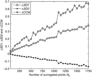

Fig. 4.3
Sensitivity of SD1, SD2 and CCM with number of shuffled points N s . At each step the number of shuffled points increased by 50. Each time the signal has been shuffled for 30 times and its mean has been taken to calculated the sensitivity
4.5.1.2 Homogeneity to Changes in Temporal Structure
In order to observe the homogeneity of sensitivity of CCM with changes in temporal structure over the whole timeline of the signal, we have used a fixed-length moving window, changed the temporal structure of that window using surrogation and then calculated CCM value of the changed signal. We have divided the signal into 20 windows with 200 samples in each of them. To minimize the bias from surrogated values, we have shuffled the points of each window 30 times and calculated all descriptors each time after shuffling. Finally, the surrogated values of descriptors were taken as a mean of the calculated values. Since we divided the entire signal into 20 windows, it resulted in 20 values of SD1, SD2 and CCM. The sensitivity of descriptors  ,
,  and
and  was calculated using Eqs. 4.10–4.11. Similar to the previous section, SD1 0, SD2 0 and CCM 0 were the parameters measured for the original data set without surrogation and j represents the window number whose data were surrogated.
 ,
,  and
and  was calculated using Eqs. 4.10–4.11. Similar to the previous section, SD1 0, SD2 0 and CCM 0 were the parameters measured for the original data set without surrogation and j represents the window number whose data were surrogated.
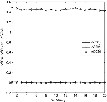
Value of  is significantly higher than
  and
and  which indicates that CCM is much more sensitive than SD1 and SD2 to the underlying temporal structure of the data (Fig. 4.4). This supports the mathematical definition of CCM as a sensitive measure of temporal variation of the signal. The little variation in
  value shows that different temporal position of changes in temporal structure does not impact the CCM value, which means the homogeneity of CCM over time. Hence, CCM reflects changes in temporal structure of the signal irrespective of the time.
 is significantly higher than
  and
and  which indicates that CCM is much more sensitive than SD1 and SD2 to the underlying temporal structure of the data (Fig. 4.4). This supports the mathematical definition of CCM as a sensitive measure of temporal variation of the signal. The little variation in
  value shows that different temporal position of changes in temporal structure does not impact the CCM value, which means the homogeneity of CCM over time. Hence, CCM reflects changes in temporal structure of the signal irrespective of the time.
