Fig. 2.1
The acquisition and reconstruction process for MR imaging. Data is collected using RF receiver coils. Through the use of time varying gradients, the data are acquired in Fourier space, also commonly referred to as k-space. A Fourier transform (FT) is required to reconstruct the desired image that displays the signal distribution in spatial coordinates
Signal Equation and k-Space
We can represent an extremely simplified MRI signal equation as:
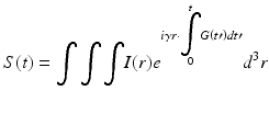
Where S(t) is the free-induction decay (FID) or echo detected by an RF receiver coil; I(r) describes the signal associated with spatial location or point r, which is dependent on several factors including proton density, T 1 and T 2 relaxation, as well as imaging parameters; i is the imaginary unit; γ is the nuclear gyromagnetic ratio; and G(t) is a vector quantity that represents the magnetic field gradient at time t after the magnetic excitation. We can then substitute:

to simplify Eq. 2.1 and we obtain:

where we can see the relationship between the acquired signal,  , the original object,
  , and the spatial-frequency distribution, k(t).

(2.1)

(2.2)

(2.3)
 , the original object,
  , and the spatial-frequency distribution, k(t).
In this notation, the signal equation which links the data acquired with the RF receiver coil to the spatial distribution of the underlying MR signal sources resembles the Fourier transform. Mapping the acquired FID to its corresponding value of  gives us our k-space representation, where the acquired time varying data is mapped onto a spatial frequency coordinate system relating it to the applied gradients. In this context, the k-space representation can be either two or three dimensional, depending on the acquisition scheme. In general, k(t) has three directional components, commonly notated as k x , k y , and k z . The acquired k-space data points are complex valued and correspond to spatial frequencies with units of 1/distance.
 gives us our k-space representation, where the acquired time varying data is mapped onto a spatial frequency coordinate system relating it to the applied gradients. In this context, the k-space representation can be either two or three dimensional, depending on the acquisition scheme. In general, k(t) has three directional components, commonly notated as k x , k y , and k z . The acquired k-space data points are complex valued and correspond to spatial frequencies with units of 1/distance.
Spatial Frequencies
The acquisition of the weighting coefficients of spatial frequencies is central to MR imaging as it is based on the concept that any image can be represented in Fourier space as a weighted sum of harmonic functions of multiple spatial frequencies and orientations. Thereby, the data representation in image space and frequency space are linked with the Fourier transform [3].
This relationship is illustrated in Fig. 2.2, where the underlying patterns of three representative spatial harmonics are explored in more detail. Datapoint (O) represents the weighting coefficient for a low spatial frequency in the ky-direction and the zero spatial frequency in the k x -direction. The spatial frequency is inversely proportional to the wavelength. Consequently, it represents a wave pattern of moderately long wavelength, λO, which is strictly oriented along the y-axis. Datapoint (P) has components in k x and k y and represents a diagonal wave pattern, here of higher spatial frequency with a shorter wavelength, λP. Datapoint (Q) is a special case as it represents the origin of the coordinate system, which corresponds to the sum of the signal in the image across all voxels, thereby reflecting the average signal intensity of the image when properly scaled. The resulting image is composed of the sum of all wave patterns weighted by the coefficient (grayscale value) in the k-space representation. It can be shown that any image can be accurately decomposed into the sum of these weighted wave patterns with varying wavelengths and angle orientations. The weighting coefficients of the wave patterns are displayed in grayscale as the k-space representation of the image.
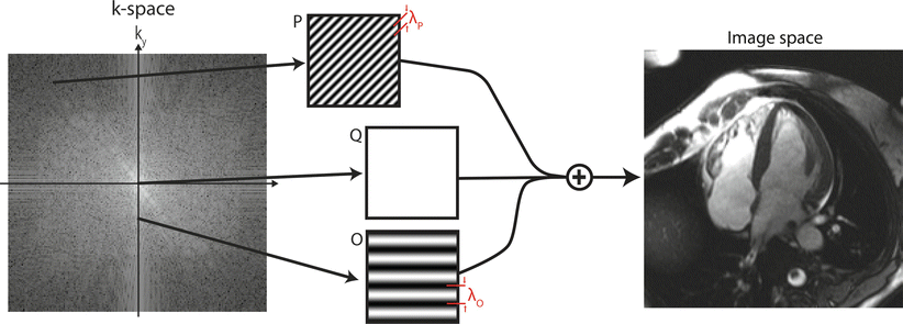

Fig. 2.2
A visual interpretation of the use of spatial harmonics to decompose an image. Every individual point in k-space represents a spatial frequency that can be represented as a wave of a certain frequency and corresponding wavelength, λ, as well as direction of the wave pattern. The image can be formed by the summation of all wave patterns weighted by their k-space coefficient, which is represented as a grayscale value in the k-space map. Representative pictures of the spatial harmonics are shown for select points O, P, and Q, with their corresponding wavelengths, λO and λP
Data Properties in Image Space and k-Space
In MRI, the k-space data, also referred to as the raw MR data, are directly measured and the corresponding image space is reconstructed by performing an inverse 2D or 3D Fourier transform. It is noteworthy that the process is reciprocal: for a known image, forward FT can generate the corresponding k-space representation, a fact that can be important for example in certain iterative reconstructions. It is further important to note that the Fourier transform generally generates complex valued data in both domains. In MR imaging, the acquired k-space signal is complex valued as it is obtained with quadrature coils containing a real and an imaginary channel. The MR image is also complex valued due to various factors including magnetic susceptibility, chemical shift, data inconsistencies from motion and flow artifacts, acquisition imperfections such as eddy currents and gradient delays, and other factors that cause the image to deviate from what would ideally be real-valued.
Consequently, a complete data representation in k-space or in image space requires the display of either the real and imaginary channel, or an equivalent display of magnitude and phase of the complex valued signal as shown in Fig. 2.3. The reconstruction process always generates a complex valued image data set. However, in most clinical scans the phase image is discarded and only the magnitude image is utilized for diagnosis. There are some exceptions where diagnostic information is contained in the phase data, including phase contrast MRI, MR elastography, susceptibility weighted imaging, spectroscopy, and fat-water imaging approaches. These techniques require the processing of the phase data in image space in addition to the magnitude data. Alternatively, the data can be stored as a real and an imaginary channel from which magnitude and phase can be derived as shown in Fig. 2.3.
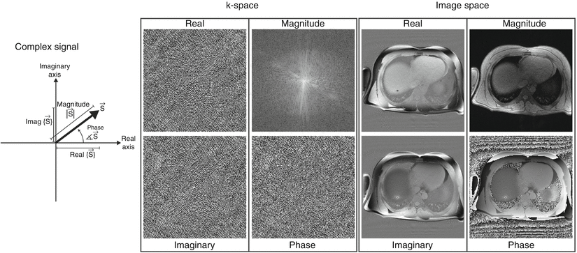

Fig. 2.3
All data from an MR system with quadrature RF coils are complex valued and can be described either by their magnitude and phase or by their real and imaginary components. Often, the image display and storage is reduced to the magnitude display. The in vivo head scan shows that an MR image is not real valued as there are phase contributions from system imperfections and effects such as magnetic susceptibility, motion, and flow
As described above, the center spatial frequency, also called the DC component because it reflects a non-varying image component similar to a direct current, represents the sum of the signal in all voxels in image space. Consequently, it is a very high signal, usually orders of magnitude higher than almost all other k-space coefficients. It is typical in MR images for most of the signal energy to be concentrated in the lower spatial frequencies because the imaging scene is dominated by large, high contrast objects. Therefore, the k-space data are commonly displayed with a logarithmic grayscale as shown in Fig. 2.4. Otherwise, the dynamic range of the display is not sufficient to distinguish signal variances in the lower signal regions, i.e., the outer regions of k-space. The k-space data are usually displayed in the form of a magnitude representation since there is little added value to the human observer to display the k-space phase, or to display the real and imaginary channels. The most essential information, namely the distribution of energy in k-space, is contained in the magnitude component. Nonetheless, it is essential for the reconstruction engine to use complex-valued k-space data and not the magnitude alone.


Fig. 2.4
k-space magnitude displays of the cardiac scan shown in Fig. 2.2 with various scaling schemes. As the center of k-space can be on the order of 10,000 times greater than the edges of k-space, a non-linear display of the grayscale can be advantageous. (a) k-space values linearly mapped to greyscale values and using the full dynamic range of the acquired data, which suppressed any signal outside the very center of k space. (b) Same as (a), except window and level settings have been changed to cap off higher signals to better appreciate lower values. (c, d) Data scaling with an exponential or logarithm scale can improve the visualization of the smaller values as seen in the higher spatial frequency components
Matrix Sizes and Artifacts
When using the Fourier transform, the matrix sizes in both domains are identical. In a 2D case, MxN k-space data points are mapped onto MxN image space data points. However, this one-to-one mapping does not always hold true as we introduce acceleration techniques, which allow us to reconstruct more image pixels from less acquired data under certain assumptions, as will be explored in greater detail in Chap. 5. It is important to note that this one-to-one mapping does not mean that a specific data point in k-space reconstructs to a specific data point in image space. In fact, each single point in k-space will influence all of the pixels in image space, because each value in k space represents a harmonic function over the whole image. This concept is essential in understanding and identifying some of the artifacts found in MRI, such as those described in Fig. 2.5.


Fig. 2.5
Errors in k-space manifest in image space based on the spatial frequencies affected. (a) If a single point in k-space is corrupt, that particular spatial frequency will appear enhanced or reduced in the reconstructed image as shown in this “corduroy” or “spiking” artifact. (b) If a patient moves during an acquisition, those portions of k-space will be corrupt and can lead to decreased image quality. These errors will be reflected in the whole image and not only in a single region of the image as shown here for illustration purposes
Properties of k-Space
The Fourier transform is a commonly used tool in signal processing for signal filtering and conditioning. Therefore, an added advantage of the k-space formalism is that the impact that parameter choices in the sampling domain have on the resulting image are well characterized by the Fourier transform properties [3]. MR imaging involves the digitization of the acquired analog RF signal. Consequently, the fundamental laws of discrete data sampling and digital signal processing apply to MR data acquisition. The Nyquist-Shannon sampling theorem describes the k-space coverage required to reconstruct an image to the desired spatial resolution, as well the maximum separation between adjacent sampling points to ensure a field-of-view (FOV) without aliasing artifact. Figure 2.6 shows the relevant relations between the digital grids in k-space and in image space for the 2D case, which are explored in more detail here.
 < div class='tao-gold-member'>


Only gold members can continue reading. Log In or Register to continue
Stay updated, free articles. Join our Telegram channel

Full access? Get Clinical Tree


