, and the other is defined as the fixed or target image . The transform defines how points from the moving image
  are mapping to their corresponding points in the fixed image
  . In three dimensional space, let
  define a voxel coordinate in the image domain of the fixed image
  . The transformation
  is a
is a  vector-valued function defined on the voxel lattice of fixed image, and
  gives the corresponding location in moving image to the point
  . The cost function represents the similarity measure of how well the fixed image is matched by a warped moving image. The optimizer is used to optimize the similarity criterion over search space defined by transformation parameters.
4D image registrations have been developed for spatial and temporal motion estimation in a 4D image sequence. 4D CT images are given as a sequence of 3D images representing different respiratory phases in the breathing cycle as discussed in Chaps. 2 and 3. Typical values are  phases from 0 to 90 % phase at 10 % intervals, where 0 % represents maximum inhale and 50 % approximately maximum exhalation. Most registration approaches use a pairwise registration paradigm, including the reference-strategy which registers each phase to a chosen reference phase (e.g. the end of expiration), and the consecutive-strategy which describes deformations respect to the neighboring time point. Figure 7.1 depicts the reference-strategy with the 50 % image as reference. For a voxel localization
  in the reference phase, the corresponding localization in the rest of the phases is given by the computed transformation, and in this way, the trajectory of a point is easily defined. Using the consecutive strategy, transformations have to be concatenated to compute a trajectory, whereby interpolation errors may be introduced.
phases from 0 to 90 % phase at 10 % intervals, where 0 % represents maximum inhale and 50 % approximately maximum exhalation. Most registration approaches use a pairwise registration paradigm, including the reference-strategy which registers each phase to a chosen reference phase (e.g. the end of expiration), and the consecutive-strategy which describes deformations respect to the neighboring time point. Figure 7.1 depicts the reference-strategy with the 50 % image as reference. For a voxel localization in the reference phase, the corresponding localization in the rest of the phases is given by the computed transformation, and in this way, the trajectory of a point is easily defined. Using the consecutive strategy, transformations have to be concatenated to compute a trajectory, whereby interpolation errors may be introduced.Fig. 7.1
Registration scheme for motion field extraction of a 4D CT data set using the reference-strategy. Each phase of the 4D CT image is registered with a chosen reference phase (e.g. the end of expiration) (figure adapted from [57])
In addition to pair-wise methods, groupwise strategies have been developed which simultaneously align multiple phases in a 4D image sequence. In these approaches, all the phase images in a 4D data set are input into the registration algorithm without assigning fixed or moving image [16, 62, 93, 99]. In this chapter, we introduce lung motion estimation from pair-wise registration between images acquired at different inflation levels.
7.2.1 Preprocessing
Many registration techniques for lung CT images require image preprocessing steps. Common preprocessing operations include downsampling large datasets, extracting region of interest (ROI), and initial pre-aligning images. As the CT imaging techniques improve, it is now possible to image lung structures with high spatial resolution, and thus produce large CT datasets. In many cases, downsampling is needed to resize the original data and to improve the registration efficiency and robustness. A further common preprocessing step is an initial alignment to roughly catch the translation, rotation, and scaling between two images, i.e. by an affine pre-registration.
One of the major challenges for registration methods in lung motion estimation is the occurrence of sliding motion between the visceral and parietal pleura (see Sect. 4.2.1) and between the individual lung lobes [4, 12, 33]. Sliding motion contradicts common regularization models applied to avoid discontinuities like gaps or foldings in the computed transformation. To cope with sliding motion, many registration methods utilize a lung segmentation mask to restrict registration to the inside of the lung. In the inter-institutional study Evaluation of Methods for Pulmonary Image Registration (EMPIRE10) [66], 16 out of 20 participating methods applied masking in at least on step of the algorithm. Due to the large density difference between the air-filled lungs and surrounding tissue, robust automatic algorithms exist for lung segmentation in CT images [52]. Figure 7.2 gives an illustration of pulmonary CT images with renderings of the lung segmentations. Image pair was acquired during breath-holds near functional residual capacity (maximum exhale) and total lung capacity (maximum inhale). Although first approaches for automatic segmentation of lung lobes exist [76, 92], lobe segmentation remains challenging because of imperceptible fissures in 4D CT images. Performing registration in the region of interest may help improve registration accuracy and efficiency, but registration is limited to the object (lung or lobe) and provides no information about other image regions. Recently, novel regularization approaches has been presented to explicitly model the sliding motion along organ boundaries (see Sect. 7.2.3.3).
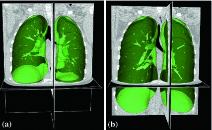
Fig. 7.2
Pulmonary CT images acquired at breath-hold (a) maximum exhale and (b) maximum inhale with renderings of the lung segmentations (green objects)
7.2.2 Similarity Criteria
Intensity-based registration utilizes the intensity information of two images to measure how well they are aligned. It takes advantage of the strong contrast between the lung parenchyma and the chest wall, and between the parenchyma and the blood vessels and larger airways. To solve the intensity-based image registration problem, it is usually assumed that intensities of corresponding voxels are related to each other in some way. Many criteria to construct the intensity relationship between corresponding points have been suggested for aligning two images, as discussed in Chap. 6. Cost functions such as mean square difference (MSD), correlation coefficient, mutual information, pattern intensity, and gradient correlation are routinely used for image registration [50, 72].
7.2.2.1 Sum of Squared Difference (SSD)
A simple and common similarity function is the sum of squared difference (SSD), which measures the intensity difference at corresponding points between two images. Mathematically, it is defined by
![$$\begin{aligned} C_{\text{ SSD }}=\int _{\varOmega } \left[ I_2({\varvec{x}})-I_1({\varvec{T}}({\varvec{x}}))\right] ^2 d{\varvec{x}}, \end{aligned}$$](/wp-content/uploads/2016/07/A217865_1_En_7_Chapter_Equ1.gif)
where  and
and  are the moving and fixed images, respectively.
  denotes the union of lung regions in fixed image and deformed moving image. The underlying assumption of SSD is that the image intensity at corresponding points between two images should be similar. This is true when registering images of the same modality. In such cases, if the images are perfectly mapped, the corresponding intensities should be identical, which means the same underlying structure has the same intensity value in the two images.
(7.1)
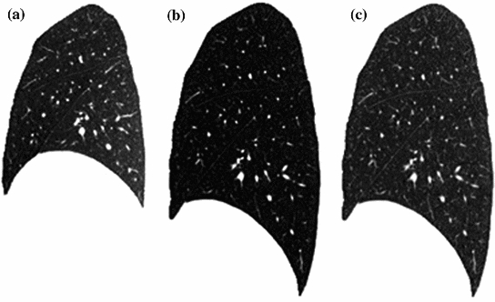
and are the moving and fixed images, respectively. denotes the union of lung regions in fixed image and deformed moving image. The underlying assumption of SSD is that the image intensity at corresponding points between two images should be similar. This is true when registering images of the same modality. In such cases, if the images are perfectly mapped, the corresponding intensities should be identical, which means the same underlying structure has the same intensity value in the two images.Fig. 7.3
Illustration of histogram matching before SSD registration between breath-hold maximum exhale and maximum inhale images from a human subject. a A sagittal slice from maximum exhale. b A sagittal slice from maximum inhale. c The sagittal slice of b after histogram modification so that its grayscale range is similar to that of a
However, considering the change in CT intensity as air inspired and expired during the respiratory cycle, the grayscale range are different within the lung region in two CT images acquired at different inflation levels. To balance this grayscale range difference, normalization of the intensities are needed. For example, a histogram matching procedure [98] can be used before SSD registration to modify the histogram of moving image so that it is similar to that of fixed image. Figure 7.3 gives an illustration of histogram matching before SSD registration between a pair of images acquired at breath-hold maximum exhale and maximum inhale from a human subject. Alternative approaches use a-priori knowledge about density changes in the lungs to preprocess images before the registration [81]. Please note that intensity normalization is only needed for SSD similarity function discussed here. It is not necessary for the similarity functions discussed below.
7.2.2.2 Similarity Functions for Multi-Modal Registration
As mentioned above, CT intensity is a measure of tissue density and therefore changes as the tissue density changes during inflation and deflation. The registration problem under this circumstance is similar to the multi-modality image registration, where similarity functions based on correlation coefficients (CC) [7, 48] or on mutual information (MI) [27, 61, 91, 94] are well suited and widely used. In the EMPIRE10 study for lung registration [66], 10 out of 20 participants used multi-modal similarity metrics based on CC or MI.
The local normalized cross-correlation (NCC) between two images  and
and  assumes a linear dependency between the image intensities and is defined by
where  iterates through a neighborhood of voxel
  and
and  is the mean value within this neighborhood.
and assumes a linear dependency between the image intensities and is defined by(7.2)
iterates through a neighborhood of voxel and is the mean value within this neighborhood.Mutual information expresses the amount of information that one image contains about the other one. Analogous to the Kullback-Leibler measure, the negative mutual information cost of two images is defined as [61, 91]
where  is the joint intensity distribution of transformed moving image
  and fixed image
  ;
;  and
and  are their marginal distributions, respectively. The histogram bins of
  and
and  are indexed by
  and
and  . Misregistration results in a decrease in the mutual information, and thus, increases the similarity cost
  . Note that the MI metric does not assume a linear relationship between the intensities of the two images (see Sect. 6.1.4.5 too). Multi-modal metrics omit the need of intensity normalization in lung registration, but the computational effort of these measures is increased compared to SSD.
(7.3)
is the joint intensity distribution of transformed moving image and fixed image ; and are their marginal distributions, respectively. The histogram bins of and are indexed by and . Misregistration results in a decrease in the mutual information, and thus, increases the similarity cost . Note that the MI metric does not assume a linear relationship between the intensities of the two images (see Sect. 6.1.4.5 too). Multi-modal metrics omit the need of intensity normalization in lung registration, but the computational effort of these measures is increased compared to SSD.7.2.2.3 Sum of Squared Tissue Volume Difference (SSTVD)
Beside the widely used standard similarity functions for mono- or multi-modal registration, a number of lung-specific similarity metrics have been developed recently.
A recently developed similarity function, the sum of squared tissue volume difference (SSTVD) [42, 102], accounts for the variation of intensity in the lung CT images during respiration. This similarity criterion minimizes the local difference of tissue volume inside the lungs scanned at different pressure levels. This criterion is based on the assumption that the tissue volume is constant between inhale and exhale.1
Assume that lung is a mixture of two materials: air and tissue/blood (non-air). Then the Hounsfield units (HU) in lung CT images is a function of tissue and air content. From the HU of CT lung images, the regional tissue volume and air volume can be estimate following the air-tissue mixture model by Hoffman et al. [49]. Let  be the volume element at location
  . Then the tissue volume
 within the volume element can be estimated as
where we assume that  and
and  . Let
. Let  and
and  be the anatomically corresponding volume elements, and
  and
and  be the tissue volumes within anatomically corresponding volume elements, respectively. Then the intensity similarity function SSTVD is defined as [101, 102]
![$$\begin{aligned} C_{\text{ SSTVD }}&= \int _{\varOmega } \left[ V_2({\varvec{x}})-V_1({\varvec{T}}({\varvec{x}}))\right] ^2 d{\varvec{x}}\nonumber \\&= \int _{\varOmega } \left[ v_2({\varvec{x}})\beta (I_2({\varvec{x}}))-v_1({\varvec{T}}({\varvec{x}}))\beta (I_1({\varvec{T}}({\varvec{x}})))\right] ^2 d{\varvec{x}}. \end{aligned}$$](/wp-content/uploads/2016/07/A217865_1_En_7_Chapter_Equ5.gif)
The Jacobian determinant (often simply called the Jacobian) of a transformation  estimates the local volume changes resulted from mapping an image through the deformation [10, 21, 25]. In 3D space, let
 ![$${\varvec{T}}(x,y,z) = [T_x(x,y,z), T_y(x,y,z), T_z(x,y,z)]^T$$](/wp-content/uploads/2016/07/A217865_1_En_7_Chapter_IEq41.gif) be the vector-valued transformation which deforms the moving image
be the vector-valued transformation which deforms the moving image  to the fixed image
  . The Jacobian of the transformation
  at location
  is defined as
Thus, the tissue volumes in image  and
and  are related by
  , and Eq. (7.5) can be rewritten as
![$$\begin{aligned} C_{\text{ SSTVD }}=\int _{\varOmega } \left\{ v_2({\varvec{x}})\left[ \beta (I_2({\varvec{x}}))-J({\varvec{T}}({\varvec{x}}))\beta (I_1({\varvec{T}}({\varvec{x}})))\right] \right\} ^2 d{\varvec{x}}. \end{aligned}$$](/wp-content/uploads/2016/07/A217865_1_En_7_Chapter_Equ7.gif)
An alternative approach based on the assumption that the total mass (tissue volume) of the lung is conserved was proposed by Castillo et al. [17], named “combined compressible local-global optical flow” (CCLG). The main idea of this approach is to substitute the conservation of mass equation for the constant intensity assumption in the classical optical flow formulation of Horn and Schunk [51].
be the volume element at location . Then the tissue volume within the volume element can be estimated as(7.4)
and . Let and be the anatomically corresponding volume elements, and and be the tissue volumes within anatomically corresponding volume elements, respectively. Then the intensity similarity function SSTVD is defined as [101, 102](7.5)
estimates the local volume changes resulted from mapping an image through the deformation [10, 21, 25]. In 3D space, let be the vector-valued transformation which deforms the moving image to the fixed image . The Jacobian of the transformation at location is defined as(7.6)
and are related by , and Eq. (7.5) can be rewritten as(7.7)
7.2.2.4 Sum of Squared Vesselness Measure Difference (SSVMD)
Feature information extracted from the intensity image is important to help guide the image registration process. During the respiration cycle, blood vessels keep their tubular shapes and tree structures. Therefore, the spatial and shape information of blood vessels can be utilized to help improve the registration accuracy. Blood vessels have larger HU values than that of parenchyma tissues. The intensity difference between parenchyma and blood vessels can effectively help intensity-based registration. However, as the blood vessel branches, the diameter of vessel becomes smaller and smaller. The small blood vessels are difficult to see because of their low intensity contrast. Therefore, grayscale information of the small vessels give almost no contribution to similarity functions directly based on intensity. In order to better utilize the information of blood vessel locations, the vesselness measure (VM) computed from intensity image can be used.
The vesselness measure is based on analyses of eigenvalues of the Hessian matrix of the image intensity. These eigenvalues can be used to indicate the shape of the underlying object. In 3D lung CT images, tubular structures such as blood vessels (bright) are associated with one negligible eigenvalue and two similar non-zero negative eigenvalues [40]. Ordering eigenvalues of a Hessian matrix by magnitude  , the Frangi’s vesselness function [40] is defined as
with
where  distinguishes between plate-like and tubular structures,
  accounts for the deviation from a blob-like structure, and
  differentiates between tubular structure and noise.
  ,
,  ,
,  control the sensitivity of the vesselness measure. In lung CT images, an example parameter setting is
  ,
,  , and
, and  .
.
, the Frangi’s vesselness function [40] is defined as(7.8)
(7.9)
distinguishes between plate-like and tubular structures, accounts for the deviation from a blob-like structure, and differentiates between tubular structure and noise. , , control the sensitivity of the vesselness measure. In lung CT images, an example parameter setting is , , and .The Hessian matrix is computed by convolving the intensity image with second and cross derivatives of the Gaussian function. For a multiscale analysis, the response of the vesselness filter will achieve the maximum at a scale which approximately matches the size of vessels to detect. Therefore, the final vesselness measure is estimated by computing Eq. (7.8) for a range of scales and selecting the maximum response:  . Here
  is the standard deviation of the Gaussian function [36].
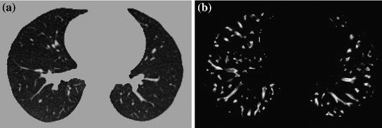
. Here is the standard deviation of the Gaussian function [36].Fig. 7.4
The vesselness images calculated from lung CT grayscale images. a A transverse slice of breath-hold maximum exhale data. b The vesselness measure of slice in a. Vesselness measure is computed in multiscale analysis and rescaled to [0, 1]
The vesselness image is rescaled to [0, 1] and can be considered as a probability-like estimate of vesselness features. Larger vesselness value indicates the underlying object is more likely to be a vessel structure, as shown in Fig. 7.4. The sum of squared vesselness measure difference (SSVMD) is designed to match similar vesselness patterns in two images. Given  and
and  as the vesselness measures of images
  and
and  at location
  respectively, the vesselness cost function is formed as [13, 14]
![$$\begin{aligned} C_{\text{ SSVMD }}&= \int _{\varOmega } \left[ F_2({\varvec{x}})-F_1({\varvec{T}}({\varvec{x}}))\right] ^2 . \end{aligned}$$](/wp-content/uploads/2016/07/A217865_1_En_7_Chapter_Equ10.gif)
Mismatch from vessel to tissue structures will result a larger SSVMD cost. This similarity metric can be used together with any other intensity-based volumetric metrics to help guide the registration process and improve matching accuracy.
and as the vesselness measures of images and at location respectively, the vesselness cost function is formed as [13, 14](7.10)
7.2.3 Transformation Constraints
Enforcing constraints on the transformation helps to generate more meaningful registration results. In general, the computed transformation should be smooth and maintain the topology of the transformed images. Furthermore, the registration method should be symmetric, and should produce the same correspondences between two images independent of the choice of fixed and moving images.
7.2.3.1 Regularization Constraints
Continuum mechanical models such as linear elasticity [22, 23] and viscous fluid [22, 24] can be used to regularize the transformations. For example, linear-elastic constraint of the form
can be used to regularize the displacement fields where
The linear elasticity operator  has the form of
  where
where ![$$\nabla = \left[ \frac{\partial }{\partial x}, \frac{\partial }{\partial y}, \frac{\partial }{\partial z} \right] $$](/wp-content/uploads/2016/07/A217865_1_En_7_Chapter_IEq68.gif) and
and ![$$\nabla ^2 = \nabla \cdot \nabla = \left[ \frac{\partial ^2}{\partial x^2} +\frac{\partial ^2}{\partial y^2} + \frac{\partial ^2}{\partial z^2} \right] $$](/wp-content/uploads/2016/07/A217865_1_En_7_Chapter_IEq69.gif) . In general,
. In general,  can be any nonsingular linear differential operator [63], e.g. a Laplacian regularization constrain is given by
Further regularization terms are discussed in Sect. 6.1.5.
(7.11)
(7.12)
has the form of where and . In general, can be any nonsingular linear differential operator [63], e.g. a Laplacian regularization constrain is given by(7.13)
The purpose of the regularization constraints are to constrain the transformation to obey the laws of continuum mechanics and ensure it maintains the topology of two images. Using a linear differential operator as defined in Eq. (7.11) can help to smooth the transformation, and to eliminate abrupt changes in the displacement fields. However, it can not prevent the transformation from folding onto itself, i.e. destroying the topology of the images under transformation [25].
To help maintain desirable properties of the moving and fixed images during deformation, another regularization example can be a constraint that prevents the Jacobian of transformations from going to zero or infinity. The Jacobian is a measurement to estimate the pointwise expansion and contraction during the deformation (see Sect. 7.2.2.3). A constraint that penalizes small and large Jacobian is given by [21]
![$$\begin{aligned} C_{\text{ Jac }}({\varvec{T}}) = \int _{\varOmega } \Bigg [(J({\varvec{T}}({\varvec{x}})))^2 + \bigg ( \frac{1}{J({\varvec{T}}({\varvec{x}}))} \bigg )^2 \Bigg ] d{\varvec{x}}. \end{aligned}$$](/wp-content/uploads/2016/07/A217865_1_En_7_Chapter_Equ14.gif)
Further examples of regularization constraints that penalize large and small Jacobians can be found in Sect. 6.1.5, and Ashburner et al. [6].
(7.14)
7.2.3.2 Inverse Consistency Constraint
In order to find better correspondence mapping and reduce pairwise registration error, one method is to jointly estimate the forward and reverse transformations between two images while minimizing the inverse consistent error.
Define forward transformation  deforms
  to
to  and the reverse transformation
  deform
  to
to  . A meaningful map between two anatomical images should be one-to-one, i.e. each point in image
  is mapped to only one point in image
  and vice versa. However, many unidirectional image registration techniques have the problem that their similarity cost function does not uniquely determine the correspondence between two images. The reason is that the local minima of similarity cost functions cause the estimated forward mapping
  to be different from the inverse of the estimated reverse mapping
  . To overcome correspondence ambiguities, transformations
  and
and  can be jointly estimated. Ideally,
  and
and  should be inverses of one another, i.e.
  . In order to couple the estimation of
  and
and  together, an inverse consistency constraint (ICC) [21] is imposed as
The constraint is minimized and the corresponding transformations are said to be inverse-consistent if  .
.
deforms to and the reverse transformation deform to . A meaningful map between two anatomical images should be one-to-one, i.e. each point in image is mapped to only one point in image and vice versa. However, many unidirectional image registration techniques have the problem that their similarity cost function does not uniquely determine the correspondence between two images. The reason is that the local minima of similarity cost functions cause the estimated forward mapping to be different from the inverse of the estimated reverse mapping . To overcome correspondence ambiguities, transformations and can be jointly estimated. Ideally, and should be inverses of one another, i.e. . In order to couple the estimation of and together, an inverse consistency constraint (ICC) [21] is imposed as(7.15)
.7.2.3.3 Sliding Preserving Regularization
The physiological characteristics of the lung motion imply discontinuities between the motion of lung and rib cage contradicting common regularization schemes. As discussed in Sect. 7.2.1, most lung-specific registration algorithms address this problem using lung segmentation masks.
Recently, novel regularization approaches were presented to explicitly model the sliding motion along organ boundaries. Ruan et al. [78] uses a regularization that preserves large shear values to allow for sliding motion. Schmidt-Richberg et al. [83] addressed sliding motion by a direction-dependent regularization at organ boundaries extending the common diffusion registration by distinguishing between normal- and tangential-directed motion. The idea of direction-dependent regularization was adopted in other publications, too [30, 71].
7.2.4 Parameterization, Optimization and Multi-Resolution Scheme
7.2.4.1 Transformation Parameterization
The transformation model defines how one image can be deformed to match another. It can be a simple rigid or affine transformation, or a non-linear transformation such as the spline-based registrations [90], elastic models [9], fluid models [19], finite element (FE) models [38], etc. The lung is composed of non-homogenous, soft tissue, interlaced by branching networks of airways, arteries, and veins. Lung tissue expansion varies within in the lung depending on body orientation, the direction of gravitation forces, the pattern of airway and vessel branching, disease conditions, and other factors. Since lung expansion is non-uniform, non-linear transformation models are needed to track tissue expansion across changes in lung volume.
To represent the locally varying geometric distortions, the transformation can be represented through different forms. There are three common parameterizations used for intensity-based registration methods of lung CT. The first type of transformation is based on B-splines, as introduced in Sect. 6.2.1. B-splines [79] are well suited for shape modeling and are efficient to capture the local nonrigid motion between two images. Considering the computational efficiency and accuracy requirement, the cubic B-Spline based parameterization is commonly chosen to represent the transformation. In the EMPIRE10 study 10 out of 20 algorithms used a B-Spline parametrization as transformation model [66]. Other basis functions such as thin-plate splines(TPS) [8], Fourier series [5], elastic body spline(EBS) [29] can also be used to parameterize the deformation.
The second type of transformation is dense deformable vector field (DVF), which is introduced in Sect. 6.2.2. The DVF is a non-parametric model representing the deformation by displacement vectors  for each voxel location. The transformation is then given by
  .
.
for each voxel location. The transformation is then given by .In the third type, the transformation is represented by a velocity field in order to ensure that the transformation is diffeomorphic. Diffeomorphisms define a globally one-to-one smooth and continuous mapping, and therefore, preserve topology and are suitable for the study of pulmonary kinematics. Given a time-dependent velocity field
 ![$${\varvec{v}}:{\varOmega }\times [0,1]\rightarrow \mathbb R ^{d}$$](/wp-content/uploads/2016/07/A217865_1_En_7_Chapter_IEq92.gif) , one defines the ordinary differential equation (ODE):
, one defines the ordinary differential equation (ODE):  , with
  . For sufficient smooth
  and fixed
  , e.g.
  , the solution
  of this ODE is known to be a diffeomorphism on
  [103]. Diffeomorphic registration algorithms are discussed in more detail in Sect. 10.4.2. Several approaches use diffeomorphic registration methods to model lung motions [28, 35, 41, 82, 86].
in order to ensure that the transformation is diffeomorphic. Diffeomorphisms define a globally one-to-one smooth and continuous mapping, and therefore, preserve topology and are suitable for the study of pulmonary kinematics. Given a time-dependent velocity field , one defines the ordinary differential equation (ODE): , with . For sufficient smooth and fixed , e.g. , the solution of this ODE is known to be a diffeomorphism on [103]. Diffeomorphic registration algorithms are discussed in more detail in Sect. 10.4.2. Several approaches use diffeomorphic registration methods to model lung motions [28, 35, 41, 82, 86].7.2.4.2 Optimization
Most registration algorithms employ standard optimization techniques to the optimal transformation, as discussed in Chap. 6. There are several existing methods in numerical analysis such as the partial differential equation (PDE) solvers to solve the elastic and fluid transformation, gradient descent, conjugate gradient method, Newton, Quasi-Newton, LBFGS, etc [56, 68, 69, 73]. One efficient optimization method is a limited-memory, quasi-Newton minimization method with bounds (L-BFGS-B) [11, 104]. It is well suited for optimization with a high dimensional parameter space. In addition, this algorithm allows bound constraints on the independent variables. For example, if the transformation are represented using B-splines, then the bound constraints can be applied on B-spline coefficients so that it is sufficient to guarantee the local injectivity (one-to-one property) of transformation [18], i.e. the transformation maintains the topology of two images. According to the analysis from Choi and Lee [18], the displacement fields are locally injective all over the domain if B-Spline coefficients satisfy the condition that  , where
  are B-Spline coefficients,
  are B-Spline grid sizes along each direction, and K is a constant approximately equal to 2.479772335.
< div class='tao-gold-member'>
, where are B-Spline coefficients, are B-Spline grid sizes along each direction, and K is a constant approximately equal to 2.479772335.Only gold members can continue reading. Log In or Register to continue
Stay updated, free articles. Join our Telegram channel

Full access? Get Clinical Tree


