, Chandan Karmakar3, Michael Brennan3, Andreas Voss4 and Marimuthu Palaniswami3
(1)
Department of Biomedical Engineering, Khalifa University, Abu Dhabi, UAE
(2)
Department of Electrical and Electronic Engineering, The University of Melbourne, Melbourne, VIC, Australia
(3)
Electrical and Electronic Engineering, The University of Melbourne, Melbourne, VIC, Australia
(4)
Department of Medical Engineering and Biotechnology, University of Applied Sciences Jena, Jena, Germany
Abstract
Physiological systems are inherently complex and subject to energy, entropy and information fluxes across their boundaries. These systems function in disequilibrium in healthy condition and their self-organizing capability is related to asymmetricity of the underlying processes (Costa et al., Phys. Rev. Lett. 95:1–4, 2005). In pathological perturbations, a loss of self-organizing capability associated with aging or disease is a function of loss of asymmetricity (Costa et al., Phys. Rev. Lett. 95:1–4, 2005). Intuitively, asymmetry refers to the lack of symmetry; in other words, the distribution of signals is imbalanced. This imbalance or dissimilarity can easily be observed in geometry of the phase space plots. Asymmetry is expected to be present in physiological systems (Chialvo and Millonas, Phys. Rev. Lett. 209:26–30, 1995) as it is the fundamental property of a non-equilibrium system (Prigogine and Antoniou, Ann. N. U. Acad. Sci. 879:8–28, 2007). Furthermore, asymmetry is linked with the time irreversibility, which is reported as highest in systems with healthy physiology (Costa et al., Phys. Rev. Lett. 95:1–4, 2005; Costa et al., Phys. Rev. Lett. 89:062102, 2002). Thus, asymmetry represents the presence of complex nonlinear dynamics in physiological signals. So far, very little work has been published in defining and measuring asymmetry in physiological signals (Piskorski and Guzik, Phys. Rev. Lett. 28:287–300, 2007).
5.1 Introduction
Physiological systems are inherently complex and subject to energy, entropy and information fluxes across their boundaries. These systems function in disequilibrium in healthy condition and their self-organizing capability is related to asymmetricity of the underlying processes [149]. In pathological perturbations, a loss of self-organizing capability associated with aging or disease is a function of loss of asymmetricity [149]. Intuitively, asymmetry refers to the lack of symmetry; in other words, the distribution of signals is imbalanced. This imbalance or dissimilarity can easily be observed in geometry of the phase space plots. Asymmetry is expected to be present in physiological systems [150] as it is the fundamental property of a non-equilibrium system [151]. Furthermore, asymmetry is linked with the time irreversibility, which is reported as highest in systems with healthy physiology [149, 152]. Thus, asymmetry represents the presence of complex nonlinear dynamics in physiological signals. So far, very little work has been published in defining and measuring asymmetry in physiological signals [153].
Heart rate variability (HRV), the variation of the time period between consecutive heartbeats, is thought to reflect the heart’s adaptability to the changing physiological conditions. HRV is a net effect of extrinsic regulation and intrinsic heart rhythm. It is however predominantly dependent on the extrinsic regulation of the heart rate [114]. The autonomic nervous system [sympathetic (SNS) and parasympathetic (PNS)] plays a major role in regulating heart rate. Sympathetic activity is responsible for increasing the heart rate while the parasympathetic activity lowers the heart rate. Both of them work concurrently to control the heart rate in a given range. In practice there is always some variability in heart rate, due to imbalances in the activity levels of SNS and PNS. Hence, any heart rate cannot increase or decrease indefinitely but instead will be followed by an opposite trend. However, it is unlikely that any increase or decrease in RR interval has a reversing effect on the very next RR interval. The speed at which the heart rate increases or decreases is variable, which implies that the periods of increasing or decreasing RR interval are also not equal. As a result, heart rate asymmetry (HRA) should be a common phenomena present in a healthy heart, which is also reported by Piskorski and Guzik [153] and Porta et al. [154] and the main focus of this chapter.
An obvious phenomenon in a typical Poincaré plot is asymmetry with respect to the line of identity (line with  slope and passes through the origin). Porta et al. have examined the asymmetry of Poincaré plot and shown the interrelationship between time reversibility, pattern asymmetry and nonlinear dynamics [154]. While doing so, the authors have used three different indices, Guzik’s index (GI), Porta’s index (PI) and Ehlers’ index (EI) [155–157]. Guzik et al. [156] analysed the asymmetry of short-segment HRV signal (5 min) and extended to long segment (30 min) [153]. It has been reported that about 80 % of healthy subjects showed HRA. Since asymmetry is a phenomenon of a healthy physiological system [149, 152], it is concluded that in a resting situation, the healthy heart should always exhibit the asymmetry.
 slope and passes through the origin). Porta et al. have examined the asymmetry of Poincaré plot and shown the interrelationship between time reversibility, pattern asymmetry and nonlinear dynamics [154]. While doing so, the authors have used three different indices, Guzik’s index (GI), Porta’s index (PI) and Ehlers’ index (EI) [155–157]. Guzik et al. [156] analysed the asymmetry of short-segment HRV signal (5 min) and extended to long segment (30 min) [153]. It has been reported that about 80 % of healthy subjects showed HRA. Since asymmetry is a phenomenon of a healthy physiological system [149, 152], it is concluded that in a resting situation, the healthy heart should always exhibit the asymmetry.
5.2 Existing Indices of HRA
The traditional asymmetry indices used in previous studies are GI, PI and EI [154–157]. For defining all the indices, let us assume that the increasing cloud I and decreasing cloud D are a set of points as shown below, respectively:
 and
and
 where M and K represent the number of points in increasing and decreasing cloud.


5.2.1 Guzik’s Index
Guzik et al. have defined the index for measuring the HRA using the Poincaré plot [156]. For defining GI, the distance of the plotted points from the line of identity is used. For ith point  of the plot, the distance can be calculated as
 P i + represents the point above the line of identity (
 ) and the distance D i is denoted as D i + , whereas P i − is the point below the line of identity, i.e.
  , and the distance is denoted by D i − . Guzik’s index (GI) is defined as

where C(P i + ) gives the number of points above the line of identity. In the new definition of asymmetry, the line of identity is not used for grouping the plotted points into two different clouds. As a result, it is not possible to calculate the new GI using Eq. 5.1. The set of points  used in Eq. 5.1 is equivalent to the increasing cloud defined in the new definition of asymmetry. Hence, using the increasing cloud I, Eq. 5.1 can be redefined using the proposed definition:

where the numerator corresponds to the increasing cloud, the denominator corresponds to the total number of points and G I p is the redefined Guzik’s index.
 of the plot, the distance can be calculated as
 ) and the distance D i is denoted as D i + , whereas P i − is the point below the line of identity, i.e.
  , and the distance is denoted by D i − . Guzik’s index (GI) is defined as
(5.1)
 used in Eq. 5.1 is equivalent to the increasing cloud defined in the new definition of asymmetry. Hence, using the increasing cloud I, Eq. 5.1 can be redefined using the proposed definition:
(5.2)
5.2.2 Porta’s Index
Porta et al. have also defined the asymmetry with respect to the line of identity [155]. Rather than considering the relative distance of the points with respect to the line of identity, the authors have assessed asymmetry by evaluating the number of points below the line of identity with respect to the overall number of points not on the line of identity. Hence, PI is defined as

According to the proposed definition, the set of points P i − is equivalent to the set of points belonging to the decreasing cloud D. Hence, Eq. 5.3 can be redefined as:

where K and M are the number of points in cloud D and I, respectively.

(5.3)

(5.4)
5.2.3 Ehlers’ Index
Ehler et al. have used the first derivative of the RR interval series for assessing asymmetry of the given distribution [157]. Skewness is measured over the first derivative signal to estimate the asymmetry of the distribution. Hence, for RR interval time series, it can be defined as

Ehlers’ index (EI) can be redefined with the proposed definition splitting into positive and negative cloud as

where
 and
and


(5.5)

(5.6)


Normalization of Indices
For the sake of comparison, normalization of the indices to a convenient scale is recommended. Both GI and PI values range between 0 and 100, with the index value of symmetry S = 50. Asymmetricity of the signal is ranked based on the difference of the index value from S. Index value > 50 represents that the distribution is positively skewed, either by the magnitude or by the number of points, whereas index value < 50 corresponds to the reverse distribution. The symmetricity in EI (![$$EI \in [-1,1]$$](/wp-content/uploads/2017/01/A273083_1_En_5_Chapter_IEq6.gif) ) is characterized as S = 0 and values > 0 or < 0 rank the asymmetricity of the signal. Therefore, to compare EI with GI and PI, it is necessary to use a normalized scale for the index value calculated. In this study, we have defined a range, R, for the index values to define asymmetricity. The range is defined as 1% of the difference between minimum and maximum index values, where i n d e x is either GI, PI or EI. Now, if i n d e x ∈ (S ± R) then the signal is symmetric, otherwise asymmetric. The redefined indices (G I p , P I p and E I p ) are also normalized in the same manner.
) is characterized as S = 0 and values > 0 or < 0 rank the asymmetricity of the signal. Therefore, to compare EI with GI and PI, it is necessary to use a normalized scale for the index value calculated. In this study, we have defined a range, R, for the index values to define asymmetricity. The range is defined as 1% of the difference between minimum and maximum index values, where i n d e x is either GI, PI or EI. Now, if i n d e x ∈ (S ± R) then the signal is symmetric, otherwise asymmetric. The redefined indices (G I p , P I p and E I p ) are also normalized in the same manner.
![$$EI \in [-1,1]$$](/wp-content/uploads/2017/01/A273083_1_En_5_Chapter_IEq6.gif) ) is characterized as S = 0 and values > 0 or < 0 rank the asymmetricity of the signal. Therefore, to compare EI with GI and PI, it is necessary to use a normalized scale for the index value calculated. In this study, we have defined a range, R, for the index values to define asymmetricity. The range is defined as 1% of the difference between minimum and maximum index values, where i n d e x is either GI, PI or EI. Now, if i n d e x ∈ (S ± R) then the signal is symmetric, otherwise asymmetric. The redefined indices (G I p , P I p and E I p ) are also normalized in the same manner.
) is characterized as S = 0 and values > 0 or < 0 rank the asymmetricity of the signal. Therefore, to compare EI with GI and PI, it is necessary to use a normalized scale for the index value calculated. In this study, we have defined a range, R, for the index values to define asymmetricity. The range is defined as 1% of the difference between minimum and maximum index values, where i n d e x is either GI, PI or EI. Now, if i n d e x ∈ (S ± R) then the signal is symmetric, otherwise asymmetric. The redefined indices (G I p , P I p and E I p ) are also normalized in the same manner.5.3 New Definition of Asymmetry in RR Interval Time Series
The line of identity in Poincaré plot is defined as the line that passes through the origin at an angle of  with x-axis. Therefore, any point P(x, y) on the line of identity can be expressed as x = y. Brennan et al. have defined the line of identity and shown that SD1 is the standard deviation perpendicular to the line of identity and SD2 is the standard deviation of plotted points along the line of identity [112]. But the mathematical formulation given for SD1 and SD2 by Brennan et al. [112] does not comply with the concept of line of identity which is shown by Piskorski and Guzik [153]. Piskorski and Guzik have also shown that the line of identity defined by Brennan et al. [112] is a line, which actually passes through the moment of inertia or centroid of the plotted data points with slope of
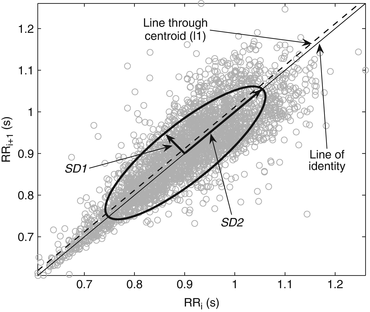
  [153]. The authors have named that line as l1 and showed the difference in calculation of SD1 and SD2 with respect to the line of identity and l1 (Fig. 5.1). The standard descriptors calculated with respect to the line of identity and l1 show negligible difference. As the line of identity has a special criteria x = y, Piskorski et al. suggested that the line of identity will be the best option for measuring SD1 and SD2. In our work, we have followed Piskorski and Guzik [153] in defining the line of identity.
 with x-axis. Therefore, any point P(x, y) on the line of identity can be expressed as x = y. Brennan et al. have defined the line of identity and shown that SD1 is the standard deviation perpendicular to the line of identity and SD2 is the standard deviation of plotted points along the line of identity [112]. But the mathematical formulation given for SD1 and SD2 by Brennan et al. [112] does not comply with the concept of line of identity which is shown by Piskorski and Guzik [153]. Piskorski and Guzik have also shown that the line of identity defined by Brennan et al. [112] is a line, which actually passes through the moment of inertia or centroid of the plotted data points with slope of
  [153]. The authors have named that line as l1 and showed the difference in calculation of SD1 and SD2 with respect to the line of identity and l1 (Fig. 5.1). The standard descriptors calculated with respect to the line of identity and l1 show negligible difference. As the line of identity has a special criteria x = y, Piskorski et al. suggested that the line of identity will be the best option for measuring SD1 and SD2. In our work, we have followed Piskorski and Guzik [153] in defining the line of identity.
Fig. 5.1
A standard Poincaré plot of RR intervals of a healthy person (N = 3000). The line of identity (solid line) and line through centroid, l1, (dashed line) are also shown. Figure adapted from Karmakar et al. [165]
The asymmetry indices GI and PI are defined based on the asymmetry definition by Piskorski and Guzik [153]. On the other hand, EI does not depend on any specific definition of asymmetry. It is directly calculated from the time-series information by computing skewness of the first derivative of the signal, i.e. the points of the Poincaré plot are not necessarily divided into two groups (increasing and decreasing). The details for calculating all indices are given in Sect. 5.4. In [153], asymmetry is defined with respect to the line of identity. All points on the line of identity (x = y) have equal consecutive RR intervals. Hence, any point above the line of identity corresponds to increasing RR interval (i.e. decreasing heart rate) and any point below corresponds to decreasing RR interval (i.e. increasing heart rate). Based on this, asymmetry is defined and quantified using different indices. Moreover, this HRA can visually be observed as the clouds of points above and below the line of identity. In healthy condition, the heart shows continuous short-term variability owing to SNS and PNS activities, which impacts on the formation of cloud around the line of identity. However, this definition of asymmetry does not represent true increasing or decreasing pattern in the heart rate. To overcome this problem, we have defined the asymmetry of heart rate in Poincaré plot independent of the line of identity, i.e. decision about a point whether it is increasing or decreasing is not made based on its position with respect to line of identity on the 2D Poincaré map. In the proposed definition, the cloud of points is partitioned into three parts: (1) points belonging to the increasing pattern of RR interval (I); (2) points belonging to the decreasing pattern of RR interval (D); and (3) points belonging to the stable pattern in RR interval (N). The decision about a point as to whether it belongs to one of the above three classes is made based on the neighbouring point in the Poincaré plot. Therefore, the analysis corresponds to at least three consecutive RR intervals of the RR interval time series for lag-1 Poincaré plot. Let the vector RR be defined as  where R R i is the ith RR interval and N is the total number of RR intervals. Furthermore, let P, the set of all points in a lag-1 Poincaré plot, be defined as
  .
.
 where R R i is the ith RR interval and N is the total number of RR intervals. Furthermore, let P, the set of all points in a lag-1 Poincaré plot, be defined as
  .
.For any two points  and
and  of the Poincaré plot, which involves three RR intervals
  , the status of the point P i + 1 with respect to clouds of points is defined as:
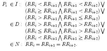
 and
and  of the Poincaré plot, which involves three RR intervals
  , the status of the point P i + 1 with respect to clouds of points is defined as:
(5.7)

Fig. 5.2
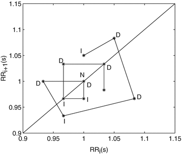
Poincaré plot points marked with cloud initials I, D and N, which indicates that the point belongs to increasing, decreasing and stable cloud, respectively. Figure adapted from Karmakar et al. [165]
After defining the clouds, the asymmetry is defined between the points of I and D, i.e. the asymmetry is defined as the lack of symmetry among the distribution of points in I and D. Hence, any point belonging to cloud N is not considered for calculating asymmetry. According to this definition, it is possible to find points I or D on both sides of the line of identity as shown in Fig. 5.2. Examples of the proposed definition with the RR intervals series shown in Fig. 5.2 are given in Fig. 5.3.
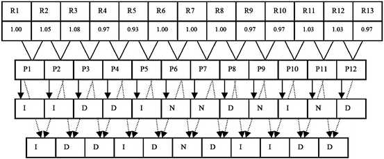

Fig. 5.3
RR interval time series of length N (= 13). The cloud type (I, D or N) corresponds to the point {P i (R R i , R R i + 1)} for Guzik’s definition and point {P i (R R i , R R i + 1), P i + 1(R R i + 1,R R i + 2)} for the new definition. Figure adapted from Karmakar et al. [165]
5.4 Modified HRA Indices Using Poincaré Plot
In this section, the asymmetry indices are redefined in accordance with the proposed definition of asymmetry. For redefining all the indices, let us assume that the increasing cloud I and decreasing cloud D are a set of points as shown below, respectively:
 and
and
 where M and K represent the number of points in increasing and decreasing cloud.


5.4.1 Guzik’s Index (G I p )
In the new definition of asymmetry, the line of identity is not used for grouping the plotted points into two different clouds. As a result, it is not possible to calculate the new GI using Eq. 5.1. The set of points  used in Eq. 5.1 is equivalent to the increasing cloud defined in the new definition of asymmetry. Hence, using the increasing cloud I, Eq. 5.1 can be redefined using the proposed definition:

where the numerator corresponds to the increasing cloud, the denominator corresponds to the total number of points and G I p is the redefined Guzik’s index.
 used in Eq. 5.1 is equivalent to the increasing cloud defined in the new definition of asymmetry. Hence, using the increasing cloud I, Eq. 5.1 can be redefined using the proposed definition:
(5.8)
5.4.2 Porta’s Index (P I p )
According to the proposed definition, the set of points P i − is equivalent to the set of points belonging to the decreasing cloud D. Hence, Eq. 5.3 can be redefined as

where K and M are the number of points in cloud D and I, respectively.

(5.9)
5.4.3 Ehlers’ Index (E I p )
Ehlers’ index (EI) can be redefined with the proposed definition splitting into positive and negative cloud as

where,
 and
and


(5.10)


5.5 Application of HRA in Clinical Research
5.5.1 Presence of HRA in Healthy Subjects
One important hypothesis about the HRA is that in resting condition a healthy heart should exhibit asymmetricity. In this section we have tested this hypothesis using both existing and redefined HRA indices.
5.5.1.1 Data and Results
In order to validate the new definition of asymmetry, GI, PI and EI using Guzik’s definition and G I p , P I p and E I p using the proposed definition of asymmetry are calculated for RR interval data of short segment (5 min) and long segment (30 min) which belongs to short-term HRV analysis [55]. The data from MIT-BIH Physionet database are used in this analysis [145]. RR intervals of 54 subjects with normal sinus rhythm (30 men, aged 28. 5–76, and 24 women, aged 58–73) have been used from the Physionet Normal Sinus Rhythm database [145] for evaluating the proposed definition. Hence we had 54 sets of recordings, of which the first 5 and 30 min were used for short- and long-segment analysis, respectively. The original long term ECG recordings were digitized at 128 Hz, and the beat annotations were obtained by automated analysis with manual review and correction [145]. The short- and long-segment RR interval series were taken from the beginning of each subject’s RR interval, but the time of the day or night cannot be mentioned as it was not clearly stated in the Physionet database. Details about the RR interval time series can be found in [158].
Stay updated, free articles. Join our Telegram channel

Full access? Get Clinical Tree


