Limited transthoracic image quality
Intra-operative assessment of ventricular function
Pre and postoperative assessment of ventricular performance
Identification of regional wall motion abnormalities suggesting ischemia
Ongoing postoperative assessment of response to medical or surgical or intervention
Evaluation of ventricular function in the critical care setting
Evaluation of unstable hemodynamics
Assessment of the integrity of the cardiac repair and its impact on ventricular function
Weaning from mechanical circulatory support
Evaluation of ventricular function during interventional cardiac catheterization procedures
Impact of procedure on ventricular performance
Imaging Planes
Optimal imaging of the left ventricle (LV) is best achieved with a combination of the transgastric mid left ventricular short axis (TG Mid SAX), transgastric long axis (TG LAX), mid esophageal four chamber (ME 4 Ch), and mid esophageal two chamber (ME 2 Ch) views [14, 15]. The miniaturization of multiplane TEE probes allows for additional imaging planes that are also quite helpful in facilitating better endocardial border definition and optimizing Doppler alignment, particularly in patients with CHD-associated with altered ventricular anatomy and geometry.
The TG Mid SAX, obtained at the mid papillary level, is the TTE equivalent of the parasternal short axis scan plane and readily facilitates the evaluation of radial ventricular function including LV shortening fraction (Fig. 5.1). This view is also optimal to evaluate regional wall motion abnormalities as all major coronary artery distributions are represented in this view.
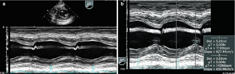
Fig. 5.1
![$ \begin{array}{c}\text{SF }\%=[\text{LVEDD}-\text{LVESD}]/\text{LVEDD}\\ =\text{[52 mm}-\text{26 mm]}/\text{53 mm}=50\%\end{array}$](/wp-content/uploads/2017/01/A125052_1_En_5_Chapter_IEq00051.gif)
Left ventricular shortening fraction. Transgastric mid short axis image at level of papillary muscles of the left ventricle (LV). (a) M-mode demonstrating left ventricular shortening. (b) M-mode derived shortening fraction (SF) of the LV:
LVEDD LV end-diastolic dimension, LVESD LV end-systolic dimension
The TG LAX view best visualizes the apex of the LV and is also helpful to assess regional wall motion. This plane, in addition to the deep transgastric long axis (DTG LAX) and sagittal (DTG Sagittal) views, allow for optimal spectral Doppler alignment with the left ventricular outflow tract, making quantitative assessment of LV cardiac output feasible.
The ME 4 Ch and ME 2 Ch views are easily obtained from the mid esophageal window. The ME 4 Ch view is most commonly used for simultaneous qualitative assessment of right ventricular (RV) and LV performance (Fig. 5.2a, b). In addition, longitudinal ventricular function is best evaluated in this view due to the optimal alignment with both lateral RV and LV walls. Overall assessment of volume status is also readily appreciated in this four chamber orientation. The ME 2 Ch view provides for biplane measurement of ventricular volume and LV ejection fraction (Fig. 5.2c, d, e).

Fig. 5.2
Left ventricular ejection fraction. Four chamber (a, b) and two chamber (c, d) views at the level of the mid esophagus in systole (a, c) and diastole (b, d). These imaging planes allow quantitative assessment of left ventricular (LV) systolic function. Simpson’s biplane methodology to calculate LV ejection fraction (e), figure adapted from Schiller et al. [16], with permission)
Echocardiographic Assessment of Global Left Ventricular Systolic Function
Echocardiographic measures of LV systolic function include M-mode, two-dimensional (2D), three-dimensional (3D), and Doppler-derived indices of ventricular performance. Each of these measures can be readily obtained with TEE [17–42]. The majority of echocardiographic measures of LV systolic function represent ejection phase indices that rely upon geometric assumptions inherent in the elliptical shape of the LV. More importantly, these measurements are significantly influenced by a variety of hemodynamic factors including altered ventricular preload and afterload, heart rate, LV mass, and myocardial contractility. The emergence of Doppler-derived measures of ventricular function has circumvented many of the geometric challenges inherent in this global assessment of ventricular performance. This is especially the case in the evaluation of RV performance as well as quantitative assessment of systolic function in patients with complex ventricular morphologies. Many of these techniques have been applied using TEE [43–51].
Left Ventricular Shortening Fraction and Fractional Area Change
One-dimensional wall motion analysis, or M-mode echocardiography, has traditionally been one of the most commonly utilized methods to measure the extent of LV shortening. Shortening fraction (SF) represents the change in LV short axis diameter that occurs during systole (Fig. 5.1):
![$ \text{LVSF}(\%)=[\text{LVEDD}-\text{LVESD}]/\text{LVEDD}\times 100$](/wp-content/uploads/2017/01/A125052_1_En_5_Chapter_Equ00051.gif) LVEDD = LV end-diastolic dimension; LVESD = LV end-systolic dimension
LVEDD = LV end-diastolic dimension; LVESD = LV end-systolic dimension
Normal values for shortening fraction range between 28 and 44 %. The LV TG Mid SAX plane is the TEE view most frequently used to make these measurements. Similar to fractional shortening, fractional area change (FAC) can also be measured in this view by determining the change in LV area that occurs during the cardiac cycle:
![$$ \begin{array}{c}\text{FAC}=\left[(\text{LV}\text{end-diastolic}\text{area})-(\text{LV}\text{end-systolic}\text{area})\right]\\ /(\text{LV}\text{end-diastolic}\text{area})\end{array}$$](/wp-content/uploads/2017/01/A125052_1_En_5_Chapter_Equ00052.gif)
Normal values have been reported to be >36 % for fractional area change in adults. LVSF and FAC have been reported to be independent of changes in heart rate and age but are significantly impacted by changes in ventricular preload and afterload [52–56].
A concern regarding this evaluation was raised in a retrospective blinded analysis comparing TTE from TEE-derived FAC measured from LV TG Mid SAX images in pediatric patients with CHD [57]. Potential errors in this measurement were reported as well as significant interobserver variability. In spite of these findings the authors were not able to exclude echocardiographic experience and training of the investigators as potential factors accounting for the variability observed. In this study, TEE-derived FAC measurement was not possible in a significant number of patients due to inability to trace endocardial borders at end-systole. Technological advances since the publication of this work may facilitate this assessment in the current era.
Left Ventricular Ejection Fraction
Left ventricular ejection fraction (LVEF) is the most commonly measured parameter of ventricular systolic function. Global estimation of LVEF is often determined in a qualitative fashion; however, utilizing TTE or TEE, 2D imaging allows quantitative measurement of LVEF by assessing changes in ventricular volume during the cardiac cycle. The geometric model most commonly used for this measurement is the modified Simpson’s biplane method (Fig. 5.2e) [16, 58–60]. By utilizing orthogonal four chamber and two chamber views of the LV (from an apical window during TTE), this geometric model calculates LV end-diastolic volume (LVEDV) and LV end-systolic volume (LVESV) by summing equal sequential slices of LV area from each of these scan planes. LVEF can then be calculated as:
![$ \text{LVEF ()}=[\text{LVEDV}-\text{LVESV}]/\text{LVEDV}\times 100$](/wp-content/uploads/2017/01/A125052_1_En_5_Chapter_Equ00053.gif)
Normal values for LVEF range between 56 and 78 %. Similar to LVSF, LVEF has been shown to be dependent on changes in ventricular loading conditions [52, 54–56, 61].
Accurate calculation of LV volume by TEE can be challenging due to foreshortening of the LV cavity. To circumvent this limitation, an area-length method to derive LVEF can also be used [24]. This method utilizes the short axis area of the LV and the long axis LV length and can be obtained by imaging the LV in the TG mid SAX and ME 4 Ch views. Determination of ventricular volume and EF by these TEE methods has been shown to correlate reasonably well with invasively measured parameters of ventricular function.
New echocardiographic technology and advancements in image processing have allowed improved acquisition of ventricular volumes. Studies have validated the ability of 3D echocardiography to obtain accurate and reproducible estimates of LV and RV volumes and EF [32–35, 62–64]. While initially limited by the time-consuming reconstruction of acquired images, advances in 3D TEE now allow for real time data display, significantly enhancing the quantitative assessment of ventricular volume and function (Chap. 19) [63, 65, 66].
Automated border detection (ABD) is another approach in imaging technology that utilizes acoustic quantification to differentiate the myocardium from the blood pool and thereby allows enhanced visualization of the endocardial border. End-diastolic and end-systolic LV area can be continuously displayed with this modality enabling determination of ventricular volume, FAC, and even pressure-volume or pressure-area loops. Excellent correlation of ABD with other noninvasive and invasive measurements of ventricular function has been reported in a few adult studies but data is lacking in patients with CHD and altered ventricular geometry [44, 46, 67–73].
Velocity of Circumferential Fiber Shortening and the Stress–Velocity Index
The rate of LV fiber shortening can be noninvasively assessed by M-mode echocardiography (a graphic display of distance over time). This measurement, termed the mean velocity of circumferential fiber shortening (Vcf), is normalized for LV end-diastolic dimension and can be obtained from the following equation:
![$ {\text{V}}_{\text{cf}}=[\text{LVEDD}-\text{LVESD}]/[\text{LVEDD}\times \text{LVET}]$](/wp-content/uploads/2017/01/A125052_1_En_5_Chapter_Equ00054.gif) LVET = LV ejection time.
LVET = LV ejection time.
Reported normal values for mean Vcf are 1.5 ± 0.04 circumferences (circ)/sec (s) for neonates and 1.3 ± 0.03 circ/s for children between 2 and 10 years of age [54, 74, 75]. This index not only assesses the degree of fractional shortening but the rate at which this shortening occurs. To normalize Vcf for variation in heart rate, LVET is divided by the square root of the R-R interval to derive a rate-corrected mean velocity of circumferential fiber shortening (Vcfc). Normal Vcfc has been reported to be 1.28 ± 0.22 and 1.08 ± 0.14 circ/s in neonates and children, respectively [54, 74–79]. Because Vcfc values are corrected for heart rate, a significant decrease in Vcfc between the neonatal and childhood age groups has been attributed to increased systemic afterload with advancing age. Vcf is sensitive to changes in contractility and afterload but relatively insensitive to changes in preload. Similar to fractional shortening, this parameter relies on the elliptical shape of the LV and is invalid with altered LV geometry.
Because the majority of ejection phase indices, including SF, EF, and Vcfc are dependent upon the underlying loading state of the LV, measures of wall tension, namely circumferential and meridional end-systolic wall stress, have been proposed to assess myocardial systolic performance in a relatively load-independent fashion [80]. Colan and colleagues have previously described a stress-velocity index that is an inverse linear relationship between Vcfc and end-systolic wall stress (Fig. 5.3). This stress-velocity index is independent of preload, normalized for heart rate, and incorporates afterload resulting in a noninvasive measure of LV contractility that is independent of ventricular loading conditions [81]. This index can therefore provide a more accurate characterization of LV myocardial systolic performance, by differentiating states of increased ventricular afterload from decreased myocardial contractility. While both conditions can affect cardiac output, the former represents increased resistance to myocardial output despite normal myocardial contractility, while the latter represents a true impairment of myocardial contractile performance. While the stress-velocity index is appealing, the clinical application of this index has been limited by its cumbersome acquisition and the need for time-consuming offline processing which are often not suitable for rapid assessment of ventricular performance such as is typically required during TEE. This index is also limited in patients with altered ventricular geometry and wall thickness, features that are hallmarks of CHD.
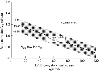
Fig. 5.3
Stress–velocity index for assessment of left ventricular systolic function. Graphic representation of the relationship between the mean rate-corrected velocity of circumferential left ventricular (LV) fiber shortening (V cfc ) and the LV end-systolic wall stress (σ es ). To normalize Vcf for variation in heart rate, it is divided by the square root of the R–R interval to derive a rate-corrected mean velocity of circumferential LV fiber shortening (V cfc ). Values above the upper limit of the mean relationship imply an increased inotropic state while values below the mean imply depressed contractility (From Colan et al. [81], with permission)
Doppler Parameters of Global Left Ventricular Systolic Function
Echocardiographic evaluation of systolic function has primarily relied upon one-dimensional measures of LV shortening or on 2D measures of LV volume changes that are often difficult to assess in patients with distorted ventricular geometry. Doppler measures of global ventricular function have been reported to be a potentially more reproducible and sensitive measure of ventricular function overcoming the limitations of other approaches.
Left Ventricular dP/dt
Doppler echocardiography can be utilized in the quantitative evaluation of LV systolic function. If mitral regurgitation (MR) is present, the peak and mean rate of change in LV systolic pressure (dP/dt) can be derived from the ascending portion of the continuous wave MR Doppler signal. This rate of change of ventricular pressure is determined during the isovolumic phase of the cardiac cycle before opening of the aortic valve. Utilizing the simplified Bernoulli equation, two velocity points along the MR Doppler envelope are selected from which a corresponding LV pressure change can be derived (Fig. 5.4). This change in LV pressure can then be divided by the change in time between the two Doppler velocities to derive the LV dP/dt. Normal values for mean dP/dt have been reported to be >1,200 mmHg/s for the LV. While more time consuming to perform, peak dP/dt correlates more accurately with invasive cardiac catheterization measurements. To ascertain peak LV dP/dt noninvasively, the MR signal is digitized to obtain the first derivative of the pressure gradient curve from which peak positive LV dP/dt can be calculated. While reflective of myocardial contractility, peak positive LV dP/dt is significantly affected by changes in preload and afterload [43, 82]. Peak negative LV dP/dt and the time constant of relaxation (Tau) can also be calculated from the MR signal, serving as indices of diastolic function.

Fig. 5.4
Left ventricular dP/dt. (a) Measurement of dP/dt. (b) Calculation of left ventricular (LV) dP/dt from the mitral regurgitation (MR) jet. This still frame demonstrates the Doppler velocity curve of the MR jet obtained during TEE in a child with dilated cardiomyopathy and severe LV dysfunction. Utilizing the simplified Bernoulli equation, the LV dP/dt is the change in LV pressure measured from 1.0 to 3.0 m/s divided by the change in time between these two LV pressure points: LV dP/dt = (36 mmHg − 4 mmHg)/63 ms = 508 mmHg/s (normal >1,200 mmHg/s). Figure 5.4a used with permission from Mayo Clinic
Myocardial Performance Index
The myocardial performance index (MPI), also referred to as Tei index, is a Doppler-derived quantitative measure of global ventricular function that incorporates both systolic and diastolic time intervals [83–87]. The MPI is defined as the sum of isovolumic contraction time (ICT) and isovolumic relaxation time (IRT) divided by ejection time (ET) (Fig. 5.5):
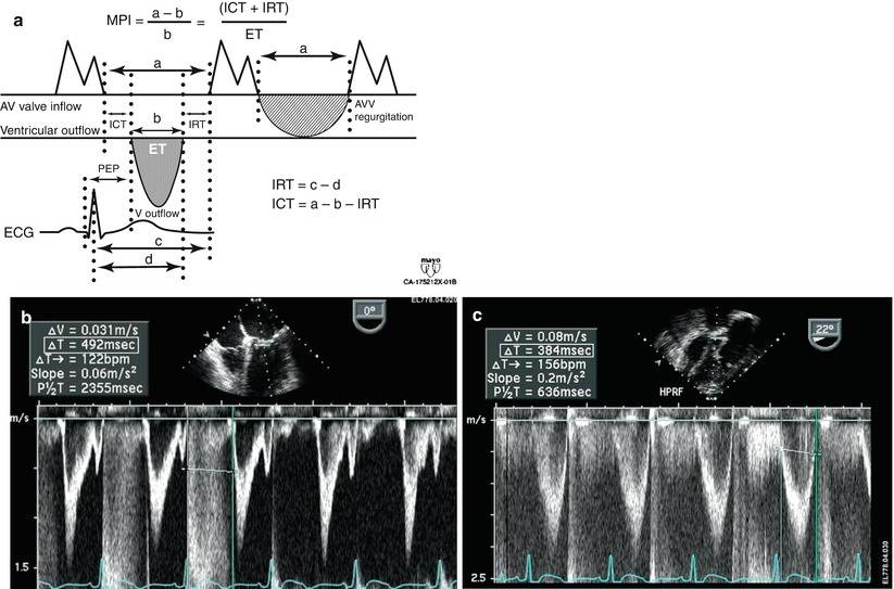
Fig. 5.5

Myocardial performance index (MPI) for assessment of left ventricular global function. AV atrioventricular, AVV atrioventricular valve, ECG electrocardiogram, PEP pre ejection period, V ventricular. (a) MPI represents the ratio of isovolumic contraction time (ICT) and isovolumic relaxation time (IRT) to ventricular ejection time (ET):
(b) Mid esophageal four chamber view. The duration of ICT + IRT is measured from the cessation of mitral valve inflow to the onset of atrioventricular valve inflow of the next cardiac cycle (interval a). (c) Deep transgastric view with pulsed wave Doppler within the left ventricular outflow tract. Ventricular ejection time is measured from the onset to cessation of LV ejection (interval b)
(Figure a from Eidem et al. [88], with permission)
The components of this index are measured from routine pulsed wave Doppler signals at the atrioventricular valve and ventricular outflow tract of either the LV or RV (as an alternative, the comparable signals from tissue Doppler imaging, as described below, can be used). To derive the sum of ICT and IRT, the Doppler derived ejection time for either ventricle is subtracted from the Doppler interval between cessation and onset of the respective atrioventricular valve inflow signal (from the end of the Doppler A wave to the beginning of the Doppler E wave of the next cardiac cycle). Increasing values of the MPI correlate with increasing degrees of global ventricular functional impairment.
Both adult and pediatric studies have established normal values for the MPI [84, 86, 88]. In adults, normal LV and RV MPI values are 0.39 ± 0.05 and 0.28 ± 0.04, respectively. In children, similar values for the LV and RV are reported to be 0.35 ± 0.03 and 0.32 ± 0.03, respectively. The MPI has been shown to be a sensitive predictor of outcome in adult and pediatric patients with acquired and CHD [85, 86, 89–94]. One of the advantages of the MPI is the ease in which it can be obtained, both by TTE as well as TEE. Because the MPI incorporates measures of both systolic and diastolic performance, this index may be a more sensitive early measure of ventricular dysfunction in the absence of other overt changes in isolated systolic or diastolic echocardiographic indices. In addition, because the MPI is a Doppler-derived index, it has been reported to be easily applied to the assessment of both LV and RV function as well as complex ventricular geometries in patients with CHD [89, 90, 92, 93]. The MPI, however, does have major limitations. It is significantly affected by changes in loading conditions, particularly preload, and has a paradoxical change with high filling pressures or severe semilunar valve regurgitation (“pseudo-normalization”). In addition, the combined nature of this index fails to readily discriminate between abnormalities of systolic or diastolic performance.
Echocardiographic Assessment of Regional Left Ventricular Systolic Function
Two-Dimensional Imaging
Regional ventricular function can be assessed by examining wall motion and systolic wall thickening. TEE, particularly in the intraoperative setting, is ideally suited for this purpose. Changes in ventricular wall motion typically occur during periods of decreased coronary perfusion, as can be the case during surgical interventions. These wall motion alterations are characterized by reduced systolic thickening and decreased inward endocardial excursion.
In order to facilitate regional wall function assessment several schemes have been proposed that include specific nomenclature, a variable number of LV segmental divisions, and different methods of wall motion analysis. Two models of LV segmental division have been favored as follows: (1) the 16-segment LV model and (2) the 17-segment LV model. The former, established in 1989 [16], represents an effort by the American Society of Echocardiography Committee on Standards and forms the basis for the recommendations in the original guidelines for performing a comprehensive intraoperative multiplane TEE examination established by the American Society of Echocardiography and the Society of Cardiovascular Anesthesiologists [95]. The latter, proposed by the American Heart Association in 2002, aimed to standardize myocardial segmentation and nomenclature for all types of cardiac imaging modalities [96]. These two models as applicable to TEE imaging are illustrated in Figs. 5.6 and 5.7.
Fig. 5.6
SCA/ASE 16-segment model of the left ventricle
Basal segments | Mid segments | Apical segments |
|---|---|---|
1. Basal antero-septal | 7. Mid antero-septal | 13. Apical anterior |
2. Basal anterior | 8. Mid anterior | 14. Apical lateral |
3. Basal lateral | 9. Mid lateral | 15. Apical inferior |
4. Basal posterior | 10. Mid posterior | 16. Apical septal |
5. Basal inferior | 11. Mid inferior | |
6. Basal septal | 12. Mid septal |
Modified from Vegas [97], with permission from Springer
Fig. 5.7
AHA 17-segment model of the left ventricle
Basal segments | Mid segments | Apical segments |
|---|---|---|
1. Basal anterior | 7. Mid anterior | 13. Apical anterior |
2. Basal antero-septal | 8. Mid antero-septal | 14. Apical septal |
3. Basal infero-septal | 9. Mid infero-septal | 15. Apical inferior |
4. Basal inferior | 10. Mid inferior | 16. Apical lateral |
5. Basal infero-lateral | 11. Mid infero-lateral | 17. Apex |
6. Basal antero-lateral | 12. Mid antero-lateral |
Modified from Vegas [97], with permission from Springer
The 16-segment model divides the LV into three levels from base to apex: basal, mid, and apical. The basal and mid levels are each divided circumferentially into six segments, and the apical level into four. The 17-segment model added the apical cap or myocardial apex at the extreme tip of the LV beyond the chamber cavity. It was also suggested that the term ‘inferior’ might be more suitable than ‘posterior’ in reference to the ventricular walls. In the most recent recommendations for chamber quantification it is pointed out that the 16-segment model is more suitable for assessing wall motion abnormalities (as the apical segment does not move), while the 17-segment model is more appropriate for myocardial perfusion evaluation and comparison among various imaging modalities [97].
The TG Mid SAX view at the level of the papillary muscles is the suggested starting point to facilitate the qualitative evaluation of regional ventricular systolic function. Although there is significant variability in the myocardial blood supply by the coronary arteries, this cross-section allows for a prompt assessment of segmental wall function since all coronary artery territories are represented in this view (Fig. 5.8). Additional TEE cross-sections are needed to evaluate all myocardial segments as allowed by multiplanar imaging, including the ME 4 Ch, ME 2 Ch, and ME LAX views (Fig. 5.8). The visual assessment of wall motion should be graded as normal/hyperkinetic, hypokinetic (reduced systolic thickening), akinetic (absent systolic thickening), dyskinetic (paradoxical systolic motion), or aneurysmal (diastolic deformation).
Fig. 5.8
Myocardial regions perfused by the major coronary arteries. The figure displays the typical myocardial territories perfused by the major coronary arteries
Left coronary circulation | Right coronary circulation |
|---|---|
Left anterior descending (LAD) artery: (anterior, antero/infero septal walls) | Right coronary artery (RCA): (inferior wall, RV, SA and AV nodes) |
Septal perforators | Posterior interventricular |
Diagonal branches | Posterior Lateral |
Posterior interventricular | Acute marginal |
Circumflex (Cx) artery: (posterior, lateral walls) | Papillary muscles blood supply: |
Obtuse marginal branches | AL by two arteries (obtuse + diagonal) |
Posterior interventricular | PM by one artery (RCA or obtuse) |
Dominance depends on which vessel (RCA or Cx) supplies the posterior interventricular branch. The majority of hearts (85 %) are right dominant. AL anterolateral, AV atrioventricular, RV right ventricle, SA sinotrial, PM posteromedial
Modified from Vegas [97], with permission from Springer
The feasibility of this segmental functional analysis and its utility has been reported in infants with CHD. In a prospective study of neonates undergoing an arterial switch operation for transposition of the great arteries, segmental wall motion was examined in the TG Mid SAX and ME 4 Ch views [98]. The presence of severe wall motion abnormalities that persisted at the completion of surgery and were present in multiple segments was found to correlate with myocardial ischemia in this cohort. This highlights the importance of regional functional analysis in patients undergoing interventions that involve the coronary arteries, aortic root or any other procedures that can potentially impact coronary perfusion.
Obviously, the two segmental models discussed apply principally to the LV in an anatomically “normal” heart—one with situs solitus, normal segments, and atrioventricular and ventriculoarterial connections (Chap. 4). As such, there will be limited direct application of these models for a number of congenital heart defects. Nonetheless the principles embodied in this segmental wall motion analysis—in particular, the evaluation of segmental wall kinetic motion—can be more generally applied to all forms of CHD. It facilitates a semi-quantitative, analytic assessment of wall motion and function even in hearts with very abnormal ventricular shape and morphology.
Tissue Doppler Imaging and Strain Rate Imaging
The assessment of regional systolic LV function, as detailed above, has centered upon the evaluation of segmental endocardial excursion and LV wall thickening. These semi-quantitative methods often fail to discriminate between active and passive myocardial motion. Newer echocardiographic modalities, including tissue Doppler imaging and strain rate imaging, offer a potentially more quantitative and accurate approach to the assessment of regional myocardial contraction and relaxation.
Tissue Doppler imaging (TDI, also known as Doppler tissue imaging or DTI) has been an addition to the armamentarium of the echocardiographer in recent years. By incorporating a high pass filter, tissue Doppler allows the display and quantitation of the low velocity high amplitude Doppler shifts present within the myocardium as opposed to the higher velocity lower amplitude Doppler signals more commonly measured within the blood pool (Fig. 5.9). Tissue Doppler echocardiography is less load-dependent than corresponding Doppler velocities from the blood pool and has systolic and diastolic components. These systolic velocities are heterogenous depending on ventricular wall and position.
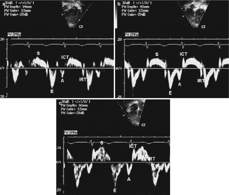
Fig. 5.9
Tissue Doppler imaging. Normal mitral annular (panel a), septal (panel b), and tricuspid annular (panel c) pulsed wave longitudinal Doppler tissue velocities. Note the characteristic normal pattern of a larger early diastolic velocity (E-wave) compared to late diastolic velocity (A-wave). The S-wave is the systolic wave. ICT, isovolumic contraction time; IRT, isovolumic relaxation time (From Eidem et al. [99], with permission)
Measurement of myocardial wall velocities by TDI has been shown to be a promising modality for assessment of longitudinal systolic performance [49, 51, 100]. Recent studies have demonstrated significant changes in mitral annular systolic TDI velocities in adult patients with LV dysfunction and elevated filling pressures [101, 102]. These indices have also been used to identify subclinical systolic ventricular dysfunction in pediatric patients [103]. Data in children following cardiac transplantation have also been found to correlate with hemodynamic parameters [104].
Tissue Doppler velocities, however, cannot differentiate between active contraction and passive motion, representing a major limitation when assessing regional myocardial function. Regional strain rate corresponds to the rate of regional myocardial deformation and can be calculated from the spatial gradient in myocardial velocity between two neighbouring points within the myocardium. Regional strain represents the amount of deformation (expressed as a percentage) or the fractional change in length caused by an applied force and is calculated by integrating the strain rate curve over time during the cardiac cycle. Strain measures the total amount of deformation in either the radial or longitudinal direction while strain rate calculates the velocity of shortening (Fig. 5.10). These two measurements reflect different aspects of myocardial function and therefore provide complementary information. In contrast to tissue Doppler velocities, these indices of myocardial deformation are not influenced by global heart motion or tethering of adjacent segments and therefore represent better indices of true regional myocardial function.
Fig. 5.10
Strain and strain rate imaging. Schematic representation of longitudinal (a) and radial (b) strain and strain rate imaging. In the longitudinal direction, strain represents myocardial shortening (systole) and lengthening (diastole) while strain rate represents the rate at which shortening or lengthening occurs. Similarly, radial strain represents myocardial thickening (systole) and thinning (diastole) while strain rate represents the rate at which thickening or thinning occurs. AVC aortic valve closure, diast diastole, MVO mitral valve opening, SR strain rate, sys systole/systolic (Figures used with permission from Luc Mertens, MD)
Studies have demonstrated regional differences in strain rate in adult patients after myocardial infarction [50, 105]. Measurements of radial and longitudinal strain rate have also been reported in normal children [106]. In addition, quantification of regional RV and LV function by strain rate and strain indexes after surgical repair of tetralogy of Fallot in children demonstrated that RV deformation abnormalities are associated with electrical depolarization abnormalities or chronic pulmonary regurgitation [107–110]. Further studies are needed to identify potential applications of strain rate imaging and related newer modalities (speckle-tracking and vector velocity imaging) in the evaluation of ventricular mechanics and regional assessment of myocardial function of both right and left ventricles in children [111]. It is hoped that future investigations can address the suitability of these approaches in the perioperative setting.
Echocardiographic Assessment of Diastolic Ventricular Function
2D and particularly Doppler echocardiography, have historically been essential noninvasive tools in the quantitative assessment of LV diastolic function. Abnormalities of ventricular compliance and relaxation can be demonstrated by characteristic changes in mitral inflow and pulmonary venous Doppler patterns [112]. Newer methodologies including tissue Doppler echocardiography and flow propagation velocities enhance the ability of echocardiography to define and quantitate these adverse changes in diastolic performance. Because diastolic dysfunction often precedes systolic dysfunction, careful assessment of diastolic function is mandatory in the noninvasive characterization and serial evaluation of patients with CHD.
Noninvasive evaluation of diastolic function in normal infants and children is influenced by a variety of factors including age, heart rate, and the respiratory cycle. Reference values detailing both mitral and pulmonary venous Doppler velocities in a large cohort of normal children have been established using transthoracic imaging [113]. Similar to many echocardiographic parameters, these Doppler velocities are also significantly impacted by loading conditions making determination of diastolic dysfunction by using these parameters alone very challenging in patients with CHD.
Although the evaluation of diastolic function using TEE has been reported in adult patients in the perioperative setting, there are no formal studies addressing this application in the pediatric age group. The discussion that follows reviews general concepts of diastolic evaluation in children with the use of echocardiography and potential applications using the transesophageal modality.
Mitral Inflow Doppler
Mitral inflow Doppler is readily obtained from the ME 4 Ch view and represents the diastolic pressure gradient between the left atrium (LA) and LV (Fig. 5.11). The early diastolic filling wave, or E-wave, is the dominant diastolic wave in children and young adults and represents the peak LA to LV pressure gradient at the onset of diastole. The deceleration time of the mitral E-wave reflects the time period needed for equalization of LA and LV pressures. The late diastolic filling wave, or A-wave, represents the peak pressure gradient between the LA and LV in late diastole at the onset of atrial contraction. Normal mitral inflow Doppler is characterized by a dominant E-wave, a smaller A-wave, and a ratio of E- and A-waves (E:A ratio) between 1.0 and 3.0. Normal duration of mitral deceleration time as well as isovolumic relaxation time vary with age and have been reported in both pediatric and adult populations [113, 115–118]. Mitral inflow Doppler velocities are not only impacted by changes in LV diastolic function but also by a variety of additional hemodynamic factors including age, altered loading conditions, heart rate, and changes in atrial and ventricular compliance. Interpretation of characteristic patterns of mitral inflow must be carefully evaluated with particular attention paid to the potential impact of each of these hemodynamic factors on the Doppler velocities.
Fig. 5.11
Doppler patterns in diastolic dysfunction. Graphic representation of spectrum of changes in mitral and pulmonary venous inflow patterns associated with diastolic dysfunction in children. A atrial filling wave, AV atrioventricular, D pulmonary vein diastolic flow wave, E early filling wave, S pulmonary vein systolic flow wave, VAR vein atrial reversal wave (Modified from: Olivier et al. [114], with permission)
The earliest stage of LV diastolic dysfunction demonstrated by mitral inflow Doppler is abnormal relaxation (Fig. 5.11). This Doppler pattern is characteristic of normal aging in adults and represents a mild decrease in the rate of LV relaxation with continued normal LA pressure. It is characterized by a reduced E-wave velocity, increased A-wave velocity, decreased E:A ratio <1.0, and a prolonged mitral deceleration time and isovolumic relaxation time (IVRT).
As diastolic dysfunction progresses, further changes in ventricular relaxation and compliance occur leading to an increase in LA pressure. Increased LA pressure normalizes the initial transmitral gradient between the LA and LV producing a “pseudo-normalized” mitral inflow Doppler pattern with increased E-wave velocity and E:A ratio, and normalized mitral deceleration and isovolumic relaxation time intervals (Fig. 5.11). This pseudo-normal Doppler pattern may be difficult to distinguish from normal mitral inflow Doppler; however, maneuvers that decrease ventricular preload, like the Valsalva maneuver, will uncover the underlying abnormalities of mitral inflow Doppler. In addition, evaluation of pulmonary venous inflow Doppler can help unmask this advanced degree of LV diastolic dysfunction (see below).
Further deterioration of LV diastolic function results in restrictive ventricular filling with an additional increase in LA pressure and a concomitant decrease in ventricular compliance. The Doppler pattern of restrictive LV filling is characterized by additional increases in E-wave velocity, reduction in A-wave velocity, an increased E:A ratio >3.0, and significant shortening of both mitral deceleration time and IVRT (Fig. 5.11) [115]. This pattern is typically seen in patients with restrictive cardiomyopathy and may also be seen in other conditions associated with restrictive physiology (i.e., acute post-transplant setting).
Pulmonary Venous Doppler
Pulmonary venous Doppler, combined with mitral inflow Doppler, provides a more comprehensive assessment of LA and LV filling pressures (Fig. 5.11) [119–121]. TEE is ideally suited to the acquisition and quantitation of pulmonary venous flows, particularly in patients with poor transthoracic windows [19, 20, 27, 122]. Pulmonary venous inflow consists of three distinct Doppler waves: a systolic wave (S-wave), a diastolic wave (D-wave), and a reversal wave that occurs with atrial contraction (Ar-wave). In normal adolescents and adults, the characteristic pattern of pulmonary venous inflow consists of a dominant S-wave, a smaller D-wave, and a small Ar-wave of low velocity and brief duration. In neonates and younger children, a dominant D-wave is often present with a similar brief low velocity, or even absent, Ar-wave.
With worsening LV diastolic dysfunction, LA pressure increases leading to diminished systolic forward flow into the LA from the pulmonary veins with relatively increased diastolic forward flow resulting in a diastolic dominance of pulmonary venous inflow (Fig. 5.11). More importantly, both the velocity and duration of the pulmonary venous atrial reversal wave are increased. Pediatric and adult studies have demonstrated that an Ar-wave duration >30 ms longer than the corresponding mitral A-wave duration or a ratio of pulmonary venous Ar-wave to mitral A-wave duration >1.2 is predictive of elevated LV filling pressure (Fig. 5.12) [113, 120]. Pulmonary venous flow variables as measured by TEE have been correlated with estimations of mean LA pressure in adults undergoing cardiovascular surgery [19].
Fig. 5.12
Mitral valve and pulmonary venous Doppler tracings. Diagram depicting mitral valve (MV) and pulmonary vein (PV) Doppler flow tracings. A atrial filling wave, A-d duration of atrial filling wave, D pulmonary vein diastolic flow wave, DT mitral deceleration time, dTVI time velocity integral of pulmonary vein diastolic flow wave, E early filling wave, ECG electrocardiogram, PVAR pulmonary vein atrial reversal wave, PVAR-d duration of pulmonary vein atrial reversal flow, S pulmonary vein systolic flow wave, sTVI time velocity integral of pulmonary vein systolic flow wave (From O’Leary et al. [113], with permission)
Tissue Doppler Imaging
Tissue Doppler imaging is particularly well suited to the quantitative evaluation of LV diastolic function and can be easily obtained by either a transthoracic or transesophageal approach. Both early (Ea) and late (Aa) annular diastolic velocities can be readily obtained by tissue Doppler echocardiography (Fig. 5.9). Similar to systolic tissue Doppler velocities, differences in diastolic velocities exist between (1) the subendocardium and subepicardium, (2) from cardiac base to apex, and (3) between various myocardial wall segments. Previous studies have reported an excellent correlation between the early annular diastolic mitral velocity and simultaneous invasive measures of diastolic function at cardiac catheterization [123]. Early annular diastolic velocities also appear to be less sensitive to changes in ventricular preload compared to the corresponding early transmitral Doppler inflow velocity [101, 123, 124]. These diastolic tissue Doppler velocities, however, are impacted by significant alterations in preload. The influence of afterload on tissue Doppler velocities is less controversial with many studies documenting significant changes in systolic and diastolic annular velocities with changes in ventricular afterload [125–127]. Therefore, the clinical use of tissue Doppler velocities in patients with valvar stenoses or other etiologies of altered ventricular afterload need to be interpreted carefully in light of this limitation.
Stay updated, free articles. Join our Telegram channel

Full access? Get Clinical Tree


