Currently, imaging assessment of patients who undergo transcatheter aortic valve implantation is based mainly on echocardiography and angiography, both limited to provide a 3-dimensional evaluation of the prosthesis within the native valve. This study involved 34 patients who underwent multislice computed tomography (MSCT) after transcatheter aortic valve implantation. Prosthesis expansion and circularity, depth of implantation, apposition degree at the ventriculoaortic junction, and positioning in relation to coronary artery ostia were evaluated. Early clinical events such as aortic regurgitation and periprocedural conduction abnormalities were recorded and correlated with multislice computed tomographic findings. MSCT provided comprehensive 3-dimensional assessments of the prostheses in 31 of 34 of patients (91%). Expansion was excellent (mean expansion ratio 100.0 ± 10.4%) and increased significantly from the ventricular side to the aortic side of the prosthesis. Circular deployment was achieved in most patients and increased from the ventricular to the aortic side. Mean implantation depth was −2.4 ± 2.5 mm, associated with a low rate (12%) of permanent pacemaker implantation. Patients with a new conduction abnormalities had the deepest prosthesis implantation, associated with lesser expansion and circularity. Perfect apposition on MSCT was associated with a low rate of significant aortic regurgitation. In conclusion, MSCT is able to provide an accurate 3-dimensional evaluation of prosthesis deployment and positioning after transcatheter aortic valve implantation. Moreover, these anatomic findings correlate with the most frequent early complications (i.e., the occurrence of aortic regurgitation and conduction abnormalities).
About 1/3 of patients with symptomatic severe valvular aortic stenosis cannot be referred to surgery because of excessive risk related to age, decreased left ventricular function, and/or extracardiac co-morbidities. In these patients, transcatheter aortic valve implantation (TAVI) has emerged as an alternative to medical treatment and balloon aortic valvuloplasty. At each step of the TAVI procedure, the role of imaging is determinant: before implantation to optimize patient selection, prosthesis sizing, and arterial access; during implantation to guide the procedure; and after implantation to assess prosthesis positioning and deployment and detect or explain complications such as aortic regurgitation (AR) or conduction abnormalities. Currently, this imaging assessment is based mainly on echocardiography and invasive angiography, which are limited in 3-dimensional assessment. Multislice computed tomography (MSCT) is gaining interest in this field because it provides a 3-dimensional assessment of the aortic root with excellent spatial and reasonable temporal resolution. Before implantation, MSCT is recommended for iliofemoral artery assessment, but its role is still debated for aortic annular diameter measurement. After implantation, MSCT provides excellent visualization of the stent frame and allows assessment of the quality of its expansion and its positioning regarding adjoining structures, but to date few studies have evaluated its interest for that purpose. The aim of our study was to evaluate the postimplantation anatomic characteristics of the Edwards SAPIEN bioprosthesis (Edwards Lifesciences, Irvine, California) with MSCT and to correlate these anatomic findings with early clinical evolution.
Methods
The institutional review board approved this study, and informed consent was waived for this retrospective study. From September 2008 to December 2009, 50 patients with severe symptomatic aortic stenosis underwent TAVI with the Edwards SAPIEN bioprosthesis in our institution. Indications for TAVI agreed with the recent consensus statement of the European Society of Cardiology and the European Association for Cardio-Thoracic Surgery : (1) effective orifice valve area ≤1 cm 2 and/or ≤0.6 cm 2 /m 2 and (2) high surgical risk estimated from a logistic European System for Cardiac Operative Risk Evaluation score >20% and/or a Society of Thoracic Surgeons score >10% or contraindication to surgery.
Among these 50 patients, 34 underwent postimplantation MSCT and were included in the study. Sixteen patients did not undergo MSCT for the following reasons: 11 because of severe renal failure, defined by creatinine clearance <30 ml/min as calculated using the Modification of Diet in Renal Disease (MDRD) formula, 3 because of postimplantation complications, and 2 because they left the hospital before MSCT could be performed.
Conduction abnormalities were electrocardiographically documented before, during, and after TAVI (at day 7 and 1 month after implantation). AR was assessed from transthoracic echocardiography at day 7 after implantation. Postprocedural AR grade ≥2 on transthoracic echocardiography and new conduction abnormality, defined as new left bundle branch block or atrioventricular block of any degree, were compared to the prosthesis deployment, positioning, and apposition as determined on MSCT.
As previously described, TAVI was performed using either the transfemoral or the transapical approaches. The transfemoral approach was performed if the minimal iliofemoral artery diameter was ≥7 mm for the 23-mm prosthesis size and ≥8 mm for the 26-mm prosthesis size. Prosthesis sizes of 23 mm (height 14.5 mm) and 26 mm (height 16 mm) were used for patients with 18- to 21-mm and 22- to 25-mm annular sizes, respectively. In our group, annular size is calculated using transthoracic echocardiography and measured in systole at the point of valve insertion on the long-axis view.
Sixty-four-detector MSCT (VCT Light-Speed 64 and HD750 Discovery; GE Healthcare, Milwaukee, Wisconsin) was performed during patient hospitalization after valve implantation (days 5 to 7). No premedication with β blockers was used to reduce heart rate before MSCT. A triphasic injection protocol was used, and 90 ml of iodixanol 320 (GE Healthcare) or iobitridol 350 (Guerbet, Villepinte, France) was injected at a rate of 5 ml/s. Retrospective electrocardiographic gating with dose modulation was used, with tube current varying from 200 mA during systole to 650 mA during diastole. Tube voltage was 100 kVp for patients with body mass indexes <25 kg/m 2 and 120 kVp for others. Axial contiguous submillimeter slices (i.e., a volume acquisition) were obtained, allowing multiplanar reconstructions and volume rendering. All raw data were reconstructed at each 10% of the RR interval from 0% to 90%.
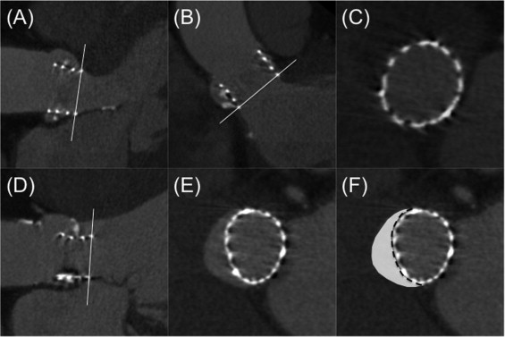
All data were transferred to a postprocessing workstation (Advantage Workstation 4.4; GE Healthcare), and analyses were performed using dedicated software (CardIQ X-Press; GE Healthcare). Two experienced observers (1 radiologist and 1 cardiologist with 5 and 3 years of experience, respectively, in cardiac computed tomography) reviewed all examinations in consensus, blinded to clinical, transthoracic echocardiographic, and angiographic data. The quality of multislice computed tomographic images was evaluated using a qualitative graduation (excellent, good, average, or poor), and the optimal diastolic phase for analysis was determined. Multiplanar reconstructions allowed us to obtain 2 left ventricular outflow tract (LVOT) views ( Figure 1 ): LVOT 1 (identical to the 3-chamber view or the parasternal long-axis view on transthoracic echocardiography) and LVOT 2 (a coronal-like view identical to posteroanterior angiographic view). Then, a double oblique transverse view was defined from the LVOT 1 and LVOT 2 views, allowing a short-axis analysis of the aortic root ( Figure 1 ).
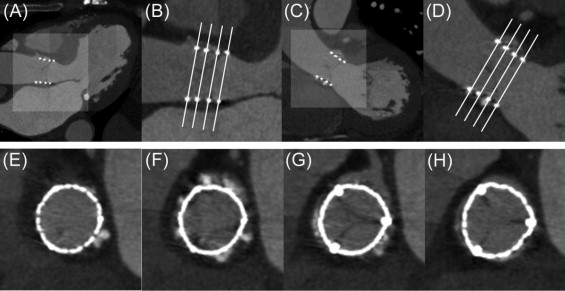
Prosthesis deployment was evaluated at 4 levels using the double oblique transverse view ( Figure 1 ) and defined as follows: level 1 was the first slice at which the frame appeared as a continuous ring at its ventricular aspect; levels 2 and 3 were the junctions between the first and second thirds and between the second and upper thirds of the frame, respectively; and level 4 was the last slice at which the frame appeared as a continuous ring on the aortic aspect of the prosthesis.
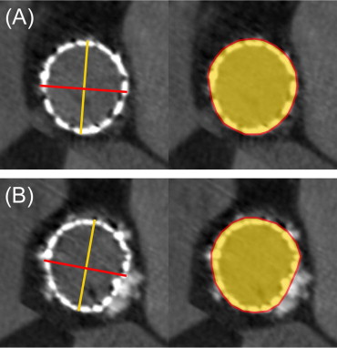
At each of these 4 levels, prosthesis deployment was assessed from 2 perspectives ( Figure 2 ): expansion and circularity. Expansion represents prosthesis deployment regarding theoretical expected surface (calculated as πr 2 , where r is half of the valve size), which depends on the valve size (415.5 mm 2 for 23-mm valve size and 531.9 mm 2 for 26-mm valve size). The expansion ratio was then deduced from the measured external short-axis area divided by the expected area and expressed as a percentage. Expansion should be as close as possible of 100%. Circularity represents the symmetry of deployment and was qualitatively evaluated using a binary visual graduation (circular or not circular) and quantitatively inferred from 2 measurements as previously described: the eccentricity index and the circularity index ( Figure 2 ). The eccentricity index was calculated as (1 − D min /D max ), where D min and D max are 2 perpendicular diameters representing, respectively, the smallest and largest external diameters at each level. A circular deployment was defined as an eccentricity index < 0.1. The circularity index was calculated as short-axis area/perimeter . For a perfect circle, the circularity index is maximal and equal to 0.079. Then, the effective circularity index was indexed to 0.079 at each level to obtain a ratio representing valve circularity.
Because visualizing the native annulus after TAVI with MSCT is difficult, implantation depth was evaluated by reference to the floor of the sinuses of Valsalva ( Figure 3 ). For each coronary sinus, the distance between the most basal point of the frame and the sinus floor was measured on multiplanar reconstruction (1) below the noncoronary sinus, to evaluate overlapping on the membranous septum; (2) below the right coronary sinus, to evaluate overlapping on the mitral valve anterior leaflet; and (3) below the left coronary sinus, to evaluate overlapping on the muscular septum. This distance was arbitrarily considered negative if the implantation was below the floor of the sinus of Valsalva and positive if above.
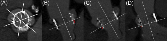
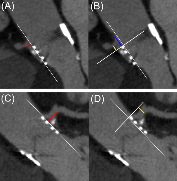
Prosthesis relation with coronary artery ostia was defined from LVOT views. The following measurements were then performed, as described in Figure 4 : the distance between the external border of the frame and the coronary ostium, prosthesis overlap above the coronary artery ostial plane (positive if covering, negative if not), and distance between the prosthesis and the sinotubular junction (positive if above, negative if not).
Apposition was assessed quantitatively at the basal level using the double oblique transverse view at level 1. The nonapposition perimeter was measured and divided by the prosthesis perimeter at level 1 to obtain a nonapposition ratio ( Figure 5 ). Nonapposition area was also measured as described in Figure 5 .
Continuous data are presented as mean ± SD or as medians with interquartile ranges if appropriate, after checking for a normal distribution using the Kolmogorov-Smirnov test. Categorical variables are presented as numbers and frequencies. Paired Student’s t tests were performed to compare continuous variables with normal distribution, whereas Mann-Whitney U tests were used in case of non-normality. Fisher’s exact tests were performed to compare categorical variables. Analyses of variance were performed to compare several means when necessary, typically for level-by-level comparison of deployment indexes. To assess relations between anatomic measurements and clinical events, we used Fisher’s exact tests and/or Mann-Whitney U tests. All statistical tests were 2 sided, and p values <0.05 were considered statistically significant. All analyses were performed using NCSS 2007 (NCSS Statistical Software, Kaysville, Utah).
Results
Baseline population characteristics and transthoracic echocardiographic data are listed in Tables 1 and 2 . The mean age was 85 ± 4.3 years, and 50% of patients were men. The mean logistic European System for Cardiac Operative Risk Evaluation score was 25.7 ± 9.2%. All aortic valves were considered tricuspid on transthoracic echocardiography. The transfemoral approach was performed in 24 patients (71%) and the transapical approach in the others. Valve size was 23 mm in 13 patients (38%) and 26 mm in 21 (62%).
| Characteristic | Value |
|---|---|
| Men/women | 17 (50%)/17 (50%) |
| Age (years) | 85 ± 4.3 |
| Body surface area (m 2 ) | 1.8 ± 0.2 |
| Logistic EuroSCORE | 25.7 ± 9.2 |
| Creatinine clearance (ml/min) | 61.7 ± 24.0 |
| Cardiovascular co-morbidities | |
| Hypertension | 22 (64%) |
| Diabetes mellitus | 7 (21%) |
| Body mass index ≥30 kg/m 2 | 7 (21%) |
| Myocardial infarction | 13 (38%) |
| Coronary artery bypass grafting | 8 (24%) |
| Percutaneous coronary intervention | 11 (32%) |
| Atrial fibrillation | 13 (38%) |
| Pacemaker | 4 (12%) |
| Stroke | 5 (15%) |
| Peripheral vascular disease | 10 (29%) |
| Noncardiovascular co-morbidities | |
| Respiratory failure | 10 (29%) |
| Chronic renal failure | 7 (21%) |
| Previous neoplasia | 8 (24%) |
| Mediastinal radiotherapy | 2 (6%) |
| Characteristic | Baseline (n = 34) | Day 7 (n = 34) | p Value |
|---|---|---|---|
| Mean left ventricular ejection fraction (%) | 56.0 ± 14.7 | 62.3 ± 10.4 | 0.045 |
| Mean pressure gradient (mm Hg) | 40.8 ± 11.9 | 10.0 ± 3.3 | <0.001 |
| Effective orifice area (cm 2 ) | 0.68 ± 0.14 | 1.75 ± 0.15 | <0.001 |
| Effective orifice area index (cm 2 /m 2 ) | 0.38 ± 0.07 | 1.0 ± 0.13 | <0.001 |
| AR grade ≥2 | 10 (29%) | 9 (26%) | 0.996 |
| Mitral regurgitation grade ≥2 | 18 (53%) | 12 (35%) | 0.221 |
| Pulmonary artery pressure (mm Hg) | 44.3 ± 15.0 | 39.5 ± 11.3 | 0.07 |
| Annular diameter (mm) | 22.0 (20.1–23.3) | — | — |
Among the 34 patients, the quality of multislice computed tomographic images was considered excellent in 20 (58.8%), good in 9 (26.5%), and average in 2 (5.9%). Three multislice computed tomographic studies (8.8%) were of poor quality and deemed noninterpretable: in 1 case, synchronization failed, and in the other 2 cases, artifacts were located in the prosthesis area. Thus, MSCT was able to provide full 3-dimensional analyses of the implanted prostheses in 31 patients (91%).
Deployment characteristics are listed in Table 3 . The mean minimal and maximal diameters were 23.2 ± 1.1 and 24.3 ± 1.1 mm for 23-mm prostheses and 24.8 ± 1.5 and 26.5 ± 1.4 mm for 26-mm prostheses, with an increase in diameter from level 1 to level 4. The mean expansion ratios were 106.5 ± 9.4% and 97.5 ± 9.6% for 23- and 26-mm prostheses, respectively. Level-by-level comparison showed a significant expansion ratio increase from the ventricular side up to the aortic side for the 2 sizes (p <0.001). Moreover, expansion ratio was significantly superior at all levels in patients with 23-mm prostheses compared with those with 26-mm prostheses.
| Variable | 23 mm (n = 12) | 26 mm (n = 19) | All (n = 31) | p Value (23 vs 26 mm) |
|---|---|---|---|---|
| Level 1 | ||||
| Minimal diameter (mm) | 22.6 ± 0.7 | 24.2 ± 1.3 | — | <0.001 |
| Maximal diameter (mm) | 24.0 ± 1.0 | 26.3 ± 1.4 | — | <0.001 |
| Eccentricity index | 0.05 (0.02–0.07) | 0.06 (0.03–0.10) | 0.06 (0.02–0.10) | 0.34 |
| Circularity index (%) | 96.5 ± 1.3 | 96.7 ± 1.5 | 96.6 ± 1.4 | 0.715 |
| Expansion ratio (%) | 101.8 ± 6.6 | 94.6 ± 7.3 | 97.4 ± 7.8 | 0.008 |
| Level 2 | ||||
| Minimal diameter (mm) | 22.6 ± 0.8 | 24.2 ± 1.4 | — | <0.001 |
| Maximal diameter (mm) | 23.9 ± 0.9 | 26.3 ± 1.5 | — | <0.001 |
| Eccentricity index | 0.05 (0.02–0.08) | 0.08 (0.03–0.11) | 0.07 (0.03–0.09) | 0.33 |
| Circularity index (%) | 96.4 ± 1.6 | 95.4 ± 1.8 | 95.8 ± 1.7 | 0.10 |
| Expansion ratio (%) | 101.6 ± 7.1 | 93.6 ± 8.5 | 96.7 ± 8.8 | 0.008 |
| Level 3 | ||||
| Minimal diameter (mm) | 23.2 ± 0.8 | 24.8 ± 1.6 | — | <0.001 |
| Maximal diameter (mm) | 24.2 ± 1.2 | 26.3 ± 1.3 | — | <0.001 |
| Eccentricity index | 0.04 (0.02–0.06) | 0.04 (0.03–0.07) | 0.04 (0.02–0.07) | 0.52 |
| Circularity index (%) | 96.6 ± 1.6 | 95.9 ± 1.5 | 96.2 ± 1.5 | 0.2 |
| Expansion ratio (%) | 106.6 ± 7.5 | 97.1 ± 9.8 | 100.8 ± 10.0 | 0.005 |
| Level 4 | ||||
| Minimal diameter (mm) | 24.3 ± 1.0 | 25.9 ± 1.4 | — | 0.002 |
| Maximal diameter (mm) | 25.2 ± 1.1 | 27.2 ± 1.4 | — | <0.001 |
| Eccentricity index | 0.03 (0.01–0.05) | 0.03 (0.01–0.05) | 0.03 (0.01–0.05) | 0.66 |
| Circularity index (%) | 95.4 ± 1.2 | 95.7 ± 1.4 | 95.6 ± 1.3 | 0.535 |
| Expansion ratio (%) | 115.9 ± 8.9 | 104.9 ± 8.8 | 109.1 ± 10.3 | 0.003 |
| All levels | ||||
| Minimal diameter (mm) | 23.2 ± 1.1 | 24.8 ± 1.5 | — | <0.001 |
| Maximal diameter (mm) | 24.3 ± 1.1 | 26.5 ± 1.4 | — | <0.001 |
| Eccentricity index | 0.04 (0.02–0.07) | 0.05 (0.03–0.10) | 0.05 (0.02–0.08) | 0.39 |
| Circularity index (%) | 96.2 ± 1.5 | 95.9 ± 1.6 | 96.0 ± 1.5 | 0.25 |
| Expansion ratio (%) | 106.5 ± 9.4 | 97.5 ± 9.6 | 100.0 ± 10.4 | 0.003 |
Deployment was visually considered circular in most cases (n = 24 [77.5%]). Using the eccentricity index, prosthesis was considered circular in 23 patients (74%) at level 1, in 25 (81%) at level 2, in 26 (84%) at level 3, and in 28 (90%) at level 4. Accordingly, a level-by-level comparison demonstrated a significant eccentricity index decrease from level 1 to level 4 for the 23-mm prosthesis (p = 0.02), as for the 26-mm prosthesis (p = 0.003), and on global analysis (p <0.001). The eccentricity index did not differ between 23- and 26-mm prosthesis size in a side-by-side comparison at each level. The mean circularity index was >95% at all levels for 23- and 26-mm prostheses and did not differ between the 2 sizes. In a level-by-level comparison, the circularity index did not significantly differ at the 4 levels, for each prosthesis size, and on global analysis.
All parameters concerning positioning are listed in Table 4 . Prosthesis implantation was below the floor of the sinuses of Valsalva in 27 patients (88%), with a mean implantation depth of −2.4 ± 2.5 mm, with no significant difference between 23- and 26-mm sizes and no difference regarding each sinus floor.


