), but their application is constrained by low spatial resolution. Hyperpolarized helium-3 or xenon-129 MR has been developed for functional imaging of pulmonary ventilation and it avoids the concern about ionizing radiation [2, 16, 23]. Xe-enhanced CT (Xe-CT) measures regional ventilation by observing the gas wash-in and wash-out rate on serial CT images [3]. Xe-CT time series are usually acquired at the same phase over several respiratory cycles with switching from room air to xenon (wash-in) or from xenon to room air (wash-out). By fitting the lung density increase (wash-in) or decrease (wash-out) over the time to single compartment exponential model, one can measure the time constant (the inverse of specific ventilation) required to reach the lung density equilibrium. But both the helium-3 and xenon gas based imaging modalities require expensive and complex equipments to either hyperpolarize or harvest the gas, which are only available in few medical centers.
Recent advances in multi-detector-row CT (MDCT), 4D CT respiratory gating methods, and image processing techniques enable us to study pulmonary function at the regional level with high resolution anatomical information compared to other methods. As discussed in Chaps.
2 and
3, MDCT can be used to acquire multiple static breath-hold CT images of the lung taken at different lung volumes, or to acquire 4DCT images of the lungs with spiral scanning using a low pitch and retrospectively reconstructed at different respiratory phases with proper respiratory control [
18,
20,
24]. Image registration can be applied to these data to estimate a deformation field that transforms the lung from one volume configuration to the other. This deformation field can be analyzed to estimate local lung tissue expansion, calculate voxel-by-voxel intensity change, and make biomechanical measurements. When combined with image segmentation algorithms [
8,
9,
11,
25], functional and biomechanical measurements can be reported on a lung, lobe, and sublobar basis, and can be used to interpret regional lung function relative to specific segments of bronchial tree. Such measurements of pulmonary function have proven useful as a planning tool during RT planning [
31] and may be useful for tracking the progression of toxicity to nearby normal tissue during RT and can be used to evaluate the effectiveness of a treatment post-therapy [
6].
Early studies using CT to study regional air volume changes have proved to enhance our understanding of normal lung function. Several groups have proposed methods that couple image registration and CT imaging to study regional lung function. Guerrero et al. have used optical-flow based registration to compute lung ventilation from 4DCT [
13,
14] with intensity-based ventilation measure. Christensen et al. used image registration to match images across cine-CT sequences and estimate rates of local tissue expansion and contraction [
5] using a Jacobian-based ventilation measure. In addition, as shown in Sect.
13.2, the intensity-based and Jacobian-based ventilation measures are based on the assumption that the regional lung volume change is due solely to air content change, which may not always be a valid assumption [
7]. Other factors, such as blood volume change, may also contribute to the regional lung volume change.
Radiation induced pulmonary diseases can change the tissue material properties of lung parenchyma and the mechanics of the respiratory system. In patients such as lymphoma, esophageal and breast cancer with reasonable functional reserve, this damage is often insignificant. However, lung cancer patients with marginal pulmonary function are at increased risk for developing symptomatic pulmonary dysfunction secondary to radiation [
22]. The regional functional lung imaging offers the opportunity to optimize the radiation therapy planning that preferentially avoid the functioning lung regions, thus potentially reducing the physiological damage. 3D conformal radiotherapy (3D CRT), intensity modulated radiotherapy (IMRT) and volumetric modulated arc therapy (VMAT) have been previously studied for the functional avoidance and showed less damage to the highly functioning lung regions when appropriate avoidance structures derived from the functional imaging were assigned to the planning system [
22,
29,
31]. Furthermore, the functional lung imaging can also be applied during the lung cancer radiation therapy to help the decision for the adaptive radiation therapy.
This chapter reviews the basic measures to estimate regional ventilation from image registration of CT images, the comparison of them to the existing golden standard and the application in radiation therapy.
13.2 Image-Registration-Based Estimates of Regional Lung Ventilation
The lung ventilation (air volume change) and perfusion (blood/tissue volume change) are the two main components of lung volume change. In order to study lung ventilation, which is part of the lung volume change, we wish to find the motion of all tissue inside the lung due to the interactions with each other caused by the change of the transpulmonary pressure. The motion of the lung tissue, can be expressed in the form of spatial function of each region of the lung if the mapping of the region between different conditions can be found. Therefore, the problem can be stated as: Given images of the lungs in two or more different conditions, find the region mapping between the different conditions.
The problem statement brings us into the realm of image registration. Image registration is the task of finding a spatial transform mapping one image into another. Many image registration algorithms have been proposed and various features such as landmarks, contours, surfaces and volumes have been utilized to manually, semi-automatically or automatically define correspondences between two images as described in Chaps.
5,
6 and
7. The basic components of the registration framework and their interconnections are shown in Fig.
7.1 of Chap.
7. As mentioned in Chap.
7, with the image registration displacement field, functional and mechanical parameters such as the regional volume change and compliance, stretch and strain, anisotropy, and specific ventilation can be evaluated.
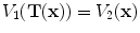
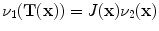
Let

and

represent two 3D image volumes to be registered. The vector
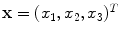
defines the voxel coordinate within an image. The algorithm finds the optimal transformation

that maps the (moving image)

to the fixed image

by minimizing the cost function defined by the user such as the combination of the similarity and the regularity. The transformation

is a

vector-valued function that maps a point

in the fixed image to its corresponding location in the moving image.
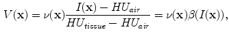
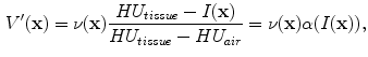
In X-ray CT based images, because the gray scale is linear between air and lung tissue, the measured Hounsfield units (HU) in the lung CT images can be assumed as a function of tissue and air content. In other words, this assumes that the lung consists only of structures equal in opacity to either air or lung tissue. Following the air-tissue mixture model by Hoffman et al. [
17], from the CT value of a given voxel, the tissue volume can be estimated as
and the air volume can be estimated as
where

denotes the volume of volume element

and

is the intensity of a voxel at position

.

and

refer to the intensity of air and tissue, respectively. Here, we assume that air is

HU and tissue is 0 HU.
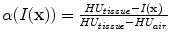
and
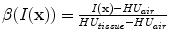
are introduced for notational simplicity. Notice that
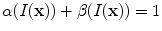
.
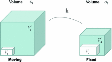
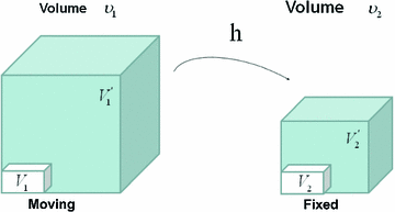
Figure
13.1 shows an example of a cubic shaped region under deformation

from moving image to fixed image. The region volumes are

and

. The volumes can be decomposed into the tissue volume fraction and air volume fraction based on the mean voxel intensity within the cube. The small white sub volumes inside the cubes represent the tissue volume

and

. Air volumes are represented by

and

(in blue). As the ratio of air to tissue decreases, the CT intensity of a voxel increases. The mean cube voxel intensities for the moving,

, and fixed images,

, are functions of the ratios of air to tissue volumes within the cubes.
13.2.1 Definition of Regional Lung Ventilation
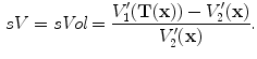
After we obtain the optimal warping function

, we can calculate the regional ventilation, which is equal to the difference in local air volume change per unit time. The commonly-used ventilation measure is the specific ventilation sV which takes the initial air volume into account. The sV is equal to the specific air volume change sVol per unit time. Or in other words, in a unit time,
Three different approaches for estimating (
13.3) are described below:
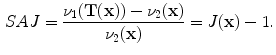
13.2.2 Specific Air Volume Change by Specific Volume Change (SAJ)
The SAJ regional ventilation measure is based on the assumption that there is no tissue volume within the moving or fixed volumes, and thus any local air volume change is equal to the local volume change. Figure
13.2 illustrates such an assumption. Compared with the general condition in Fig.
13.1, the region volume now is pure air volume, or equivalently,

and

. In this case, the specific air volume change is equal to specific volume change. Since the Jacobian tells us the local volume expansion (or contraction), the regional ventilation can be measured by:
Previously, SAJ has been used as an index of the regional function and was compared with Xe-CT estimates of regional lung function [
25] which is the local ventilation time constants calculated by observing the gas wash-in and wash-out rates on serial CT images. Regional lung expansion, as estimated from the Jacobian of the image registration transformations, was well correlated with xenon CT specific ventilation [
8,
25] (linear regression, average

).
Since the SAJ does not depend on the air-ratio which may not be available in some modalities, it can be applied to non-X-ray CT images, such as hyperpolarized He-3 MRI [
10], as long as the regional transformation of the lung tissue is known.
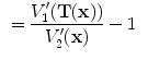
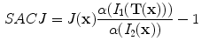
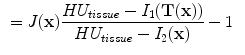
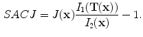
13.2.3 Specific Air Volume Change by corrected Jacobian (SACJ)
Starting with (
13.4) and expressing the air volumes

and

using the air-tissue mixture model (
13.1) and (
13.2), we obtain the corrected Jacobian measure of region air volume change, SACJ,
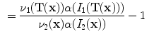
The notation

is interpreted as the image

deformed by the transformation

and is computed using linear interpolation. The deformed volume element

is calculated using the Jacobian

times the volume element

, i.e.,

. The specific air volume change is then
If we assume that pure tissue is 0 HU, then specific air volume change is
Compared to Eq.
13.4, the term

is a correction factor that depends on the voxel intensities in the moving and fixed images. The SAJ is a special case of SACJ where tissue volume is assumed to be 0, or the air volume fraction
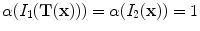
. The SACJ measure is illustrated in Fig.
13.1, and represents the most general case of where there is both tissue volume and air volume change within the region.
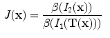
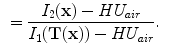
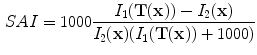
13.2.4 Specific Air Volume Change by Intensity Change (SAI)
The intensity-based measure of regional air volume change SAI can be derived from the SACJ by assuming that tissue volume is preserved during deformation, or equivalently, that the tissue volume difference
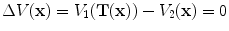
. Under this assumption,
and we have
and
Since
, with above equation, we have
Substituting the above equation into Eq.
13.9, yields
Finally, if we assume that pure air is

HU and pure tissue is 0 HU, then
which is exactly the result from Simon [
26], Guerrero et al. [
14], and Fuld et al. [
12].
Figure
13.3 illustrates the assumption with no tissue volume change in SAI. In Fig.
13.3 as the region volume changes from

to

, the tissue volume inside the cube remains the same (

).
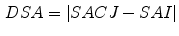
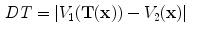
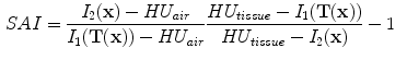
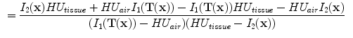
13.2.5 Difference of Specific Air Volume Change (DSA) and Difference of Tissue Volume (DT)
To investigate the relationship between the measurements of specific air volume changes and the tissue volume change, we can calculate the difference between Eqs. (
13.9) and (
13.16) and define the difference of specific air volume change (DSA) between SACJ and SAI, and the difference of tissue volume (DT) as:
 from moving image to fixed image.
  and
and  are tissue volumes in the regions.
  and
and  are air volumes in the regions. Region volumes
  and
and 
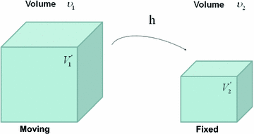
 from moving image to fixed image, with the assumption of no tissue volume (
 ).
).  and
and  are air volumes
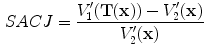
 from moving image to fixed image, with the assumption of no tissue volume change. Notice the tissue volume
  under this assumption.
  and
and  are air volumes