Estimating Internal Respiratory Motion from Respiratory Surrogate Signals Using Correspondence Models

Fig. 9.1

An illustration of how a correspondence model is typically built. Prior to treatment one or more respiratory surrogate signals are acquired simultaneously with imaging data. The motion of the internal anatomy is measured from the imaging data, e.g. using deformable image registration. A correspondence model is then fit which approximates the relationship between the internal motion and the surrogate signal(s)

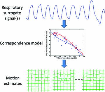
Fig. 9.2

An illustration of how a correspondence model is typically used. During RT treatment the respiratory surrogate signal(s) can be easily measured. The correspondence model can then be used to estimate the internal motion corresponding to the measured surrogate signal(s). These motion estimates could then be used to guide gated or tracked treatments

Correspondence models have also been proposed for other applications including motion compensated image reconstruction in Cone-Beam CT (CBCT) [37, 54, 69] (cf. Sect. 14.5) and Positron Emission Tomography (PET) [38] and for other image guided interventions such as High Intensity Focussed Ultrasound (HIFU) and cardiac catheterisation. For example, to perform motion compensated CBCT reconstruction a correspondence model can be built from 4D CT, which relates the motion of the anatomy to the displacement of the diaphragm. When the CBCT data is acquired the diaphragm motion can be measured from each individual projection. The correspondence model can then be used to estimate the motion for each projection, enabling a motion compensated reconstruction to be performed. A recent review paper [47] which covers all aspects of using correspondence models to estimate respiratory motion includes a description of the various different applications that have used such models.

Establishing accurate and robust correspondence models can be very challenging and is still very much an open area of research. Issues such as hysteresis, where the tumour follows a different path during inhalation and exhalation, and phase offsets between the tumour motion and the surrogate motion, may mean that a simple linear correlation between the surrogate signal and the tumour motion is insufficient to accurately predict the tumour motion [1, 2, 8, 16, 24, 28, 34, 39, 53]. Another problem is that it is well known that there can be breath to breath variations (inter-cycle variation) in the respiratory motion, both during a single fraction of treatment (intra-faction variation) and between fractions of treatment (inter-fraction variation) [24, 48]. Therefore the correspondence models need to account for or adapt to the variations in the respiratory motion.

The rest of the chapter is arranged as follows: Sect. 9.2 will review different respiratory surrogate signals that have been used for correspondence model in the literature; Sect. 9.3 will review different methods used to image the internal motion and different representations of the motion used for correspondence models; Sect. 9.4 will review the correspondence models that have been used in the literature; Sect. 9.4.2 will review methods of fitting the correspondence models to the data; and Sect. 9.5 will discuss some of the issues raised by the previous sections and the problems that still need to be overcome before the correspondence models can enter widespread clinical use.

9.2 Respiratory Surrogate Signals

Many different respiratory surrogate signals have been used for correspondence models. This section will give a brief overview of some of the most common surrogate signals that have been used in the literature. Note, surrogate signals are also used in 4D CT reconstruction to sort the imaging data into coherent volumes (cf. Part I).

Spirometers are used to measure the volume (or flow) of air being inhaled and exhaled by the patient. Spirometry is a popular choice of respiratory surrogate signal [24, 27, 41–43, 68, 71] as the signal is physiologically related to the respiratory motion and has historically been used for assessing respiratory performance and patterns [3]. However, it has been reported that some patients can have difficulty tolerating spirometry for long periods of time [24], and that spirometry measurements can be subject to time dependent drifts of the end-exhale and end-inhale values due to escaping air and instrumentation errors [24, 27, 43]. One solution to this problem is to use another ‘drift-free’ surrogate signal to correct for the drifts [43].

Another popular choice of respiratory surrogate signal is to measure the displacement of the patient’s chest or abdomen. This is often done using one or more Infra-Red (IR) markers which are tracked optically [2, 8–15, 21, 23, 25, 37, 38, 43, 45, 46, 49, 57–60, 64, 66], and there are a number of commercial system that use this technology: e.g. the Real-Time Position Management (RPM) system (Varian, Palo Alto, California, USA), the Cyberknife (Accuray, Sunnyvale, California, USA), and the ExacTrac system (Brainlab, Feldkirchen, Germany). Other methods of tracking the displacement of the chest or abdomen include electromagnetic tracking systems [24], laser tracking systems [4, 28, 55, 61], and respiratory belts which go around the patient’s chest or abdomen and stretch with respiration, e.g. the Anzai respiratory gating system (Siemens, Erlangen, Germany).

Another option for measuring the displacement of the chest and abdomen is to acquire a 3D representation of the patient’s skin surface over the chest and abdomen. This has been done using stereo imaging techniques (e.g the Align RT system, Vision RT, London, UK) [26, 27, 44, 48], and the use of time of flight cameras has also been proposed [17]. For building the correspondence models the skin surface can be extracted from CT [15, 17, 19, 35, 45, 46] or MR volumes [20], although another method will be required to monitor the surface during treatment. The displacement at different points on the surface or over different areas of the surface can be followed and used as surrogate signals [15, 17, 19, 20]. Alternatively, a single, global, surrogate signal can be produced by calculating the volume underneath the skin surface [44, 48], which has been shown to produce a similar signal to that acquired from a spirometer but without the signal drift that can affect spirometry [27, 35].

Surrogate signals measured from the internal anatomy have also been proposed in the literature. Such signals may be more closely related to the motion of the tumour and other internal anatomy, but are much more challenging to measure during RT treatment. The motion of one or more points on the diaphragm can be used as surrogate signals [5–7, 32, 33, 54, 69, 70]. During treatment diaphragm position could be followed using x-ray imaging (although imaging dose could be a factor) [6, 7] or using ultrasound imaging [67]. It has also been proposed that the lung surface could be used as a surrogate signal [40], although it is not clear how the full lung surface would be detected during RT treatment delivery.

It should be noted that a number of correspondence models use derived surrogate signals as well as the measured surrogate signals. These include processing the surrogate signal to calculate the respiratory phase, a time-delayed copy of the surrogate signal, and the temporal derivative of the surrogate signal. Using respiratory phase can be useful for modelling hysteresis, but if respiratory phase is used on its own then it is not possible to model any inter-cycle variation. Using the time derivative of a surrogate signal, or a time delayed copy of the surrogate signal, in conjunction with the original signal can enable the modelling of hysteresis and some degree of inter-cycle variation.

Some authors have proposed using full 2D images of the internal anatomy (e.g. CBCT projection data) as surrogate data [36, 65]. When using full images as the surrogate data, the direct relationship between the surrogate data and the internal motion is not modelled. Rather, an ‘in-direct’ correspondence model is used to estimate the internal motion from the surrogate data (cf. Sect. 9.4.3).

9.3 Internal Motion Data

9.3.1 Imaging the Internal Motion

This section will describe the different imaging modalities that have been used in the literature for imaging the internal respiratory motion. Some papers image the respiratory motion and construct the correspondence models at the same time as planning the RT treatment, i.e. several days before the treatment. Other papers image the respiratory motion just prior to treatment with the patient setup ready for treatment. This means that a new model can be built for each fraction of treatment and can help account for inter-fraction variations in the respiratory motion (cf. Sect. 9.5). Figure 9.3 shows examples of the different types of imaging data that have been used to image the motion of the internal anatomy.

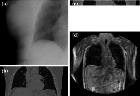
Fig. 9.3

Examples of the different types of imaging data that have been used to image the respiratory motion of the internal anatomy. a An x-ray projection image, b a 4D CT volume, c a Cine CT volume, d a dynamic MRI volume (acquisition time approx 250 ms for the full volume)

Dynamic x-ray imaging (such as fluoroscopy ) has been used to image the internal respiratory motion [1, 4, 6, 7, 9–11, 14, 24, 25, 28, 29, 44, 55, 57–61, 64, 66] (cf. Fig. 9.3a). Its main advantages are that it can be easily acquired just prior to or during RT treatment and can be acquired with a very high temporal resolution so that the images can be considered free of motion artefacts. However, as noted in the introduction to this chapter, it can be very difficult to detect the tumour in x-ray images due to it being occluded by high intensity structures such as bones or the mediastinum. One solution is to implant small radio-opaque markers into or close to the tumour in order to follow its motion [4, 9–11, 14, 25, 28, 29, 55, 57, 58, 61, 64]. These markers are easily detectable in the x-ray images and can be automatically tracked, but have a number of drawbacks including an invasive procedure to implant them and the possibility of them moving away from their intended locations [50, 62]. Therefore developing methods to automatically determine the tumour motion from x-ray images without using implanted markers is an active area of research [44, 60]. As x-rays produce 2D projection images two simultaneous x-ray images from different directions are generally required to track the 3D motion. Another option that has been proposed is to use a series of x-ray images acquired with the source and detector rotating around the patient, i.e. the raw projections images from a cone-beam CT acquisition (cf. Chap. 14). The model can then be fit to all of the x-ray images simultaneously, allowing the full 3D motion to be modelled [44].

CT imaging has been widely used in the literature to image the internal respiratory motion. It provides information on the full 3D motion and deformation of the anatomy, enabling 3D deformable registrations to be performed. Many studies have used 4D CT datasets as described in Part I to image the respiratory motion during free breathing [2, 15–19, 32, 33, 36–38, 40, 54, 65, 69, 70] (cf. Fig. 9.3b). These are popular as they provide images over the full region of interest. However, they are formed by combining data acquired from several different respiratory cycles, and are based on the assumption that the respiratory motion will be the same from one respiratory cycle to the next. Breath-to-breath variations in the respiratory motion will cause artefacts in the 4D CT volumes (cf. Sect. 1.5.1 and Sect. 2.5). This also means that 4D CT volumes are not appropriate for studying and modelling the short term breath-to-breath variations in the respiratory motion.

To overcome this problem some studies have used Cine CT data [8, 12, 21, 23, 41, 42, 45, 46, 48, 49, 68, 71] (cf. Fig. 9.3c) which is essentially the unsorted data used to construct cine 4D CT volumes (cf. Chap. 2). This means that the field of view and number of slices in the superior-inferior direction is limited by the size of the CT detector. Many scanners used clinically only have 12 or 16 slices covering approximately 2-2.5 cm. Some recently developed scanners can have a much larger detector giving greater coverage and many more slices [51], although these are still not generally large enough to cover the whole region of interest for RT planning. Therefore, if motion estimates are required for the whole region of interest it may be necessary to build multiple correspondence models and to combine the results from these models [45, 46, 48, 49, 68]. Cine CT data may be acquired at the same location over more than one respiratory cycle, giving information on the breath-to-breath variations that occur.

MRI data has also been used for constructing correspondence models [5, 20, 34, 39, 53] (cf. Fig. 9.3d). MRI has the advantage that it does not deliver any radiation dose to the patient, potentially allowing much more data to be acquired so as to study both the intra- and inter-fraction variation, and enabling volunteer studies. It is possible to acquire 3D MR volumes of a large region of interest (e.g. the lungs) at a temporal resolution fast enough to image the respiratory motion (0.5 s per image), although the spatial resolution and image quality is poor compared to 4D CT making accurate image registration much more challenging [5, 20].

9.3.2 Representing the Internal Motion Data

Some papers just model the motion of one or a small number of points of interest. In a clinical setting the point of interest would usually correspond to the tumour. Some papers manually determine the motion of the point of interest but most papers use an automatic method such as template tracking (e.g. [41]). Other correspondence models estimate the motion over an entire region of interest. In these cases image registration is often used to determine the motion from the imaging data. Affine registrations have been used [5], although deformable registrations are more common as these can account for the local deformations that occur during respiration. Several different deformable registration algorithms have been used in the literature, including B-spline (e.g. [46]), demons (e.g. [36]), optical flow/diffusion (e.g. [70]), fluid (e.g. [40]), and surface based registrations (e.g. [33]). For more information on the different registration algorithms please see Part II.

All correspondence models in the literature essentially represent the internal motion data using a motion vector, $\mathbf{m}=\left[ m_{1},m_{2},\dots ,m_{N_m}\right] ^T$ , where there are $$N_m$$

values representing the internal motion. In some cases the elements of the motion vector correspond to the motion of one or more anatomical points. These could be a point of interest such as the tumour [1, 2, 6–11, 13, 14, 24, 25, 28, 29, 34, 39, 41, 42, 44, 55, 57–61, 64, 71], or they could be points defining the surface of an organ [5, 32, 33]. The actual values used could correspond to the absolute position of the points (in some predefined coordinate system) or the displacement of the points relative to a reference position [33]. Some papers only model the 1D motion (usually in the SI direction) of the anatomical points, so $\mathbf{{m}}=\left[ x_{1},x_{2},\dots ,x_{N_p}\right] ^T$ where $x_{n}$ is the motion of the $$n$$

th point and $$N_p$$

is the number of anatomical points. In this case $$N_m=N_p$$

. Some papers model the 2D motion of the anatomical points so $\mathbf{{m}}=\left[ x_{1},y_{1},x_{2},\dots ,x_{N_p},y_{N_p}\right] ^T$ and $$N_m=2N_p$$

, and some papers model the full 3D motion of the points so $\mathbf{{m}}=\left[ x_{1},y_{1},z_{1},x_{2},\dots ,x_{N_p},y_{N_p},z_{N_p}\right] ^T$ and $$N_m=3N_p$$

, where $x_{n}$ is the motion of the $$n$$

th point in the x direction, $y_{n}$ is the motion of the $$n$$

th point in the y direction, and $z_{n}$ is the motion of the $$n$$

th point in the z direction.

Table 9.1

Summary of the different types of correspondence models used in the literature

Type	Details	Examples
Linear	1 surrogate signal	[1, 2, 6–9, 11, 16, 24, 25, 28, 34, 39, 53, 55, 57–61]
	2 or more surrogate signals	[6, 7, 10, 13–15, 17, 19, 20, 29, 32, 33, 40–42, 44, 48, 55, 68–71]
Piece-wise linear	1 surrogate signal	[21, 23]
	Using respiratory phase as surrogate signal	[54]
Polynomial	1 surrogate signal	[13, 25, 45, 55]
	With separate inhalation and exhalation	[5, 13, 14, 25, 48, 61, 64]
	2 surrogate signals	[55, 64]
B-spline	Using respiratory phase as surrogate signal	[12, 45, 46, 48, 49]
	2 or more surrogate signals	[18]
Others	Fourier series	[45]
	Neural networks	[29, 64]
	Fuzzy logic	[64]
	Support vector regression	[13, 14]

Other representations of the motion have also been used in the literature. The motion vector could represent a deformation field [15, 17, 19, 36–38, 40, 54, 65, 68–70], where each element of $\mathbf{m}$ corresponds to the motion of a voxel in a particular direction, and $$N_m$$

equals 3 times the number of voxels in the volume. The motion vector could represent a velocity field that defines a diffeomorphic transformation [21, 23], where each element of $\mathbf{m}$ corresponds to the velocity at a voxel in a particular direction, and $$N_m$$

again equals 3 times the number of voxels in the volume. Or the motion vector could represent a control point grid defining a B-spline transformation [12, 18, 20, 45, 46, 48, 49], where each element of $\mathbf{m}$ corresponds to the displacement of one of the control points in one direction and $$N_m$$

equals 3 times the number of control points that define the B-spline transformation. The size of the motion vector, $$N_m$$

, will depend on the motion representation being used. It will be small if only one or a few points of interest are being modelled, it could be several thousand if points defining an organ surface are being modelled, it could be many thousand if a B-spline control point grid is being modelled, or it could be millions if a deformation or velocity field is being modelled.

9.4 Correspondence Models

9.4.1 Types of Model

This section will describe some of the different correspondence models that have been used to relate the internal motion to respiratory surrogate signals. Table 9.1 summarises the different correspondence models that have been used in the literature. Figure 9.4 illustrates the different motion trajectories that can be modelled by the more popular types of correspondence models in Table 9.1.

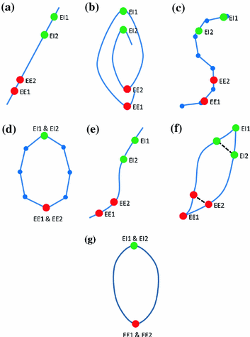
Fig. 9.4

Examples of the different motion trajectories that can be produced by the different types of correspondence model. The points corresponding to end-exhalation (red circles) and end-inhalation (green circles) from two breath cycles are marked (EE1, EI1, EE2, EI2). a A linear correspondence model using one surrogate signal constrains the motion to follow a straight line during every breath cycle. The estimated motion may move a different distance along the line during each breath, depending on how deep the breathing is (i.e. EE1 $\ne$ EE2 and EI1 $\ne$ EI2). b A linear (or other) correspondence model that uses two or more surrogate signals can model complex motion including hysteresis (a different trajectory during inhalation and exhalation) and inter-cycle variation (EE1 $\ne$ EE2 and EI1 $\ne$ EI2). c A piece-wise linear model produces a motion trajectory that is made up of several straight line segments. The blue circles correspond to known motion measurements made from the imaging data. As with the linear model, the estimated motion is constrained to follow the same path during every breath, but may move a different distance along the path depending on how deeply the individual is breathing. d If the surrogate signal used for the piece-wise linear model is a derived respiratory phase signal rather than the actual measured surrogate signal then the line segments will form a loop shaped trajectory. In this case the estimated motion will go around the same loop during every breath cycle. This means that hysteresis can be modelled, but inter-cycle variation cannot (i.e. EE1 $$=$$

EE2 and EI1 $$=$$

EI2). e A polynomial correspondence model also constrains the motion to follow the same path during every breath, but now the path is a curve rather than one or more straight lines. f In order to model hysteresis some authors have proposed using two polynomial models, one for inhalation and one for exhalation. While this does allow hysteresis to be modelled it may result in discontinuous motion estimates when switching between the two models, as shown at EE2 and EI2. g Using respiratory phase as the surrogate signal and a periodic B-spline correspondence model gives a similar trajectory to using phase with a piece-wise linear model, but the trajectory is now a smooth curve rather than being composed of a number of straight line segments

9.4.1.1 Linear Models

As can be seen in Table 9.1, linear correspondence models are by far the most common in the literature. These model the motion as a linear combination of surrogate signals:

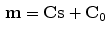
$\begin{aligned} \mathbf{{m}} = \mathbf{{Cs}} + \mathbf{{C}_\mathbf{{0}}} \end{aligned}$

(9.1)

where $\mathbf{m}$ is the vector of motion estimates (see Sect. 9.3.2), $\mathbf{s}$ is a vector of surrogate signals (i.e. $\mathbf{s}=\left[ s_1,s_2,\dots ,s_{N_s}\right] ^T$ where $$s_n$$

is the

th surrogate signal and there are $$N_s$$

surrogate signals, some of which may be derived surrogate signals), $\mathbf{C}$ is a $N_m \times N_s$ matrix of linear coefficients, and $\mathbf{C_0}$ is a $$N_m$$

element vector of constant terms.

Several papers use a linear model with just a single surrogate signal (i.e. $$N_s=1$$

), which is therefore a simple linear correlation between the surrogate signal and the motion. This constrains the motion to follow a straight line during each breath (cf. Fig. 9.4a). Such a model was first proposed for RT related applications by Schweikard et al. [57] for guiding tracked RT treatment using the Cyberknife (Accuray, Sunnyvale, California, USA). Although such a model may not be very realistic, it has been shown to be sufficiently accurate in some circumstances, and is used clinically in the Cyberknife system to treat some patients [25, 61].

There have been a number of studies assessing how different factors can affect the correlation between the surrogate signal and the motion [1, 2, 8, 16, 24, 28, 34, 39, 53], e.g. the surrogate signal used [24], the type of breathing the patient is performing (deep or shallow, using their ribs or using their diaphragm) [34, 53], and over what time scales the linear correlations are valid [24]. These studies have had mixed results. In some circumstances a simple linear correlation can approximate the respiratory motion relatively well over a short time frame, but in other circumstances, such as when there is significant hysteresis, a simple 1-D linear correlation is not sufficient.

Other papers have used linear models of two or more (sometimes many more) surrogate signals (i.e. $$N_s>1$$” src=”/wp-content/uploads/2016/07/A217865_1_En_9_Chapter_IEq42.gif”></SPAN>). When there are only two signals these usually comprise one measured surrogate signal and one derived surrogate signal, either a time delayed signal or the temporal derivative (e.g. [<CITE><A href=

$$N_s>1$$” src=”/wp-content/uploads/2016/07/A217865_1_En_9_Chapter_IEq42.gif”></SPAN>). When there are only two signals these usually comprise one measured surrogate signal and one derived surrogate signal, either a time delayed signal or the temporal derivative (e.g. [<CITE><A href=

41]). When more signals are used they are often multiple measured surrogate signals from different parts of the anatomy (e.g. [32]), although sometimes they will use multiple measured and multiple derived signals (e.g. [20]), and sometimes just a single measured signal with multiple derived signals (i.e. a number of time delayed signals with a different length delay for each signal, e.g. [29]). Sometimes the different signals may be highly correlated with each other, e.g. when the signals represent points on the surface of an organ, and this can make the models susceptible to over-fitting [32, 33]. However, the models are very flexible and can potentially model complex motion including both hysteresis and inter-cycle variation (cf. Fig. 9.4b). Linear models using multiple surrogate signals were first proposed for RT related applications by Low et al. [41].

One way to model more complex motion with only a single surrogate signal is to use a piece-wise linear model [21, 23, 37, 38, 54]. In this case the motion has been measured from several images (e.g. using deformable image registration), each of which corresponds to a different surrogate signal value. These motion measurements are linearly interpolated to estimate the motion at other surrogate signal values where data has not been acquired. Such models allow the motion to follow more complex paths than a simple straight line, but as with any model using a single surrogate signal, they are limited in the variation they can model. A piece-wise linear model that relates the motion to the measured surrogate signal [21, 23] cannot model hysteresis but can model some limited inter-cycle variation. The motion will always follow the same trajectory during each breath, but can move a different distance along this trajectory depending on how deeply the patient is breathing (cf. Fig. 9.4c). A piece-wise linear model that relates the motion to respiratory phase [37, 38, 54] can model hysteresis but cannot model any inter-cycle variation (cf. Fig. 9.4d). Furthermore, a piece-wise linear model cannot extrapolate outside the range of surrogate signal values used to build the model.

< div class='tao-gold-member'>

Only gold members can continue reading. Log In or Register to continue

Stay updated, free articles. Join our Telegram channel

Tags: 4D Modeling and Estimation of Respiratory Motion for Radiation Therapy

Jul 1, 2016 | Posted by admin in RESPIRATORY | Comments Off

Thoracic Key

Fastest Thoracic Insight Engine

Estimating Internal Respiratory Motion from Respiratory Surrogate Signals Using Correspondence Models

9.2 Respiratory Surrogate Signals